Download
1 / 42
420 likes | 569 Views
Phylogenetic inference or “How to recognize a tree from quite a long way away”. Slides are available on the course’s web page. Mikael Thollesson Evolutionary Biology Centre, Uppsala University. “Bioinformation in the cell”. RNA. polypeptide. DNA. mRNA. enzyme. protein. coenzym

E N D
Phylogenetic inferenceor “How to recognize a tree from quite a long way away” Slides are available on the course’s web page Mikael Thollesson Evolutionary Biology Centre, Uppsala University
“Bioinformation in the cell” RNA polypeptide DNA mRNA enzyme protein coenzym activation protein folding transcription splicing translation
“Extended bioinformation” Original sense strand Original sense strand New anti-sense strand New sense strand Original anti-sense strand Original anti-sense strand
111 110 Phylogeny from a Bioinformatic viewpoint • A phylogeny is the (event) history more or less exclusively shared by some kind of biological replicators • These replicators can in practice be for example • Species, population, strains • Genomes, genes • Populations • Phylogenies can usually be modelled as trees; phylogeny and phylogenetictree has thus become more or less synonymous, even though it is not • The objective for phylogenetic analysis is to infer these history and events, usually resulting in a phylogenetic hypothesis in the form of a tree (together with cosmology the only science dealing with particular histories) 010 000
Parallel substitutions and multiple substitution at the same site creates ambiguities about the hierarchy We must make some a priori assumption of homology – for sequences, this is the same as doing a multiple alignment Ordering the sequences hierarchically after shared evolutionary novelties, synapomorphies, produce a phylogenetic hypothesis (tree) We can not distinguish between novelties and ancestral state, just see the difference GCCACaTTCcCGAgCA GCCACaTTCcCGATCA GCCACaTTCcCGAgCA GCgACTagCGCGATCA GCCACaTTCcCGATCA GCCACaTTCcCGATCA GCgACTTTCcCGATtA GCgACTTTCGCGATta GCgACTagCGCGATCA GCgACTagCGCGATCA GCgACTTTCcCGATtA GCgACTTTCGCGATCA GCgACTTTCGCGATtA GCgACTTTCGCGATta ? GCgACTTTCGC--Tta GCCACTTTCGCGATCA Time
Characters Taxa, Terminal units Character states Bullfrog Cod Lion Whiteshark Bald eagle limbsamnion Lion yes yes Bald eagle yes yes Bullfrog yes no Cod no no Whiteshark no no
Pd Mv Ma Lg Pd Ma Mv Lg Pd Lg Ma Mv Pd Pd Pd Ma Mv Lg Ma Lg Ma Mv Mv Lg Mi. akkeshiensis Li. geniculatus My. versicolor Pa. dubius 22 27 26 27 27 Mv Pd Ma Lg Mv Ma Pd Lg Mv Lg Ma Pd 22 26 27 22 26 Lg Mv Ma Pd Lg Ma Mv Pd 3. Find the tree that best fit the data and choose it to be the preferred hypothesis 26 27 22 22 22 26 Lg Pd Ma Mv Ma Lg Pd Mv Ma Mv Pd Lg Ma Pd Mv Lg Lineus geniculatus TGGGCTGGGATGAAGGGAAGTATCGTGGGCCCGG MicruraakkeshiensisGGGGCTAGAATGAATGGGA-TAACGAGCCCCCGA Myoisophagus versicolor GGGGCTAGAATGAAAGAAA-GTTTGAGACCTCAT Parvicirrus dubius GGGACTGGAATGAAAGAAA-TTTTGAGGCCTTAA 1. Gather data from the entities whose phylogeny we are interested in 95% 4. Evaluate the sampling variation in the data to see if you have enough support for your conclusion 2. Select a criterion to evaluate how well each possble tree fits the observed data
Why do phylogenetics? – Prediction • Prospective biomedical compounds from sponges (Porifera) • Treatment of microsporidia • Gauging biodiversity for conservation “Taxa are not related because of similarity, but similar due to relatedness”
Why the oaks retain their leaves in contrast to other deciduous trees Evolution of metabolic pathways Tracing infection histories for virus Evergreens Why? –Sequence of evolutionary events
Why? – (Ab)use of comparative method Correlation between ability to fly and being black and white Species, populations, or genes (i.e., entities corresponding to replicators) are not independent samples/observations since they have a more or less inclusively shared history
Terminal nodes (external vertices) represent taxa or genes on which we have observations Internal vertices represent inferred splitting events (may be interpreted as ancestral species or gene copies) Unrooted vs. rooted trees A D C A B D B C e1 e2 clade e3 e6 e4 e5 Trees and terminology A branch or edge C B D D node or vertex Rooting is normally done using a designated outgroup
X is defined to be more closely related to Y than to Z if and only if X shares a (more recent) history with Y that it does not share with Z Relatedness A C B D B A C D D C A B
Collect your data Select an optimality criterion (“Which tree is better”?) Optional: do data transformations (“corrections”) Select a search strategy and find the best hypothesis (according to selected criterion) using this search method Assess the variation in your data in some way There are really only two big theoretical problems in phylogenetic inference… The criterion and calculating the score Finding the best tree “The standard recipe” for phylogenetic inference
Step 1 – Data collection Any observation of inherited traits is in principle useful Primary homology assessment - from traits to characters and character states; for sequence data this corresponds to alignment Pair-wise differences (e.g., DNA-DNA hybridization, histocompatibility) can also be used, although with a limited set of criteria Include one or several outgroups for rooting
Assumptions in shared by (almost) all optimality criteria/methods • Characters are independent (and thus the order in the data matrix does not matter) • Special models for e.g., rRNA and codons • The substitution process is homogenous over time/in the entire tree (overall rate can vary) • Special models do not make this assumption • Substitution rates are the same for all characters • Can be accommodated easily in most methods
Parsimony optimality criterion Given two trees, the one requiring the lowest number of character changes necessary to explain the observed character distribution is the better Parsimony score for a tree is the minimum number of required changes This score is frequently referred to as number ofsteps or tree length The method can be modified using non-uniform weights Character weights (positional weights) Character state weights (transformational weights)
Total tree length: 7 Total tree length: 8 Total tree length: 8 Parsimony – an example aacgtatgga bacgggtgca gaacggtgga daactgtgca a: c g: a a: c g: a a: c g: a b: c d: a d: a b: c b: c d: a
Using substitution models – Why? Jukes-Cantor is the simplest model in a class of models called time-reversible (GTR) models for DNA GTR (most complex symmetric model) has six different rates (one for each pair of bases) and different base frequencies Observed differences A G C T Actual changes , if i≠j , if i=j Example: Jukes-Cantor model P(t)=eQt
pgd= pdg=2/10=0.2 (p distance) – Jukes-Cantor distance Pair-wise distances – an example aacgtatggac bacgggtgcac gaacggtggac daactgtgcac
Minimum evolution optimality criterion Starts by calculating pair-wise distances between all terminal taxa/sequences These calculations can incorporate explicit substitution models, e.g., Jukes-Cantor Given two trees, the one having the lowest sum of branch lengths when fitted to the data, is the better One way to fit the data is using the constraints below, or using least squares approximation No branch can have negative length, eij≥0 The path between two terminals along the tree is at least as long as the pair-wise distance, eij≥dij The score is commonly referred to as tree length (as for parsimony)
Maximum likelihood optimality criterion Given two trees, the one with the higher likelihood, i.e. the one with the higher conditional probability of observing the data, is the better Site likelihood is the conditional probability of the data at one site (one character) given the assumed model of evolution and parameters of the model Data set likelihood is the product of the site likelihoods (character independence) Likelihood values under different models are comparable, thus giving us a way to test the adequacy of the model The model consists of A substitution model, e.g. Jukes-Cantor A tree with branch lengths
at Taxon1 AC Taxon2 CC For Jukes-Cantor! Ltot=L1·L2, or log Ltot = logL1+logL2 Likelihood of a one-branch tree Taxon1 AC Taxon2 CC
Another one-branch tree at at= 0.02327 lnL= -51.133956 lnL 30 nucleotides from yh-globin genes of two primates on a one-edge tree * * Gorilla GAAGTCCTTGAGAAATAAACTGCACACTGG Orangutan GGACTCCTTGAGAAATAAACTGCACACTGG There are two differences and 28 similarities
Likelihoods of a more interesting tree… Bases at internal nodes are unknown A C e1 e3 e5 u v e2 e4 A T
Number of (rooted) trees for n terminals is (2n-3)·(2n-5)·(2n-7)…3·1 3 taxa -> 3 trees 4 taxa -> 15 trees 10 taxa -> 34 459 425 trees 25 taxa -> 1,19·1030 trees 52 taxa -> 2,75·1080 trees Finding the optimal tree is an NP-complete or NP-hard problem Search strategies Exact Will find the best (according to selected criterion) tree Exhaustive Up to ca 10 taxa Branch and bound Up to ca 15 taxa Heuristic Limits the search to a “reasonable” set of trees. May not find the optimal tree Step 3 – Finding the best tree
Heursitic tree searches usually start with hill climbing (greedy algorithms) to obtain a starting tree Star decomposition Stepwise addition and proceed with some flavour of branch swapping to improve on the starting tree and find better trees
Heursitic tree search – Star decomposition A A A B A C C C E D D E B B E D C E D C E B D B A … E A B A E E C C C A B B D D D
Heursitic tree search – Stepwise addition B A C A B B A A C 831 837 E D A C B D D C C 783 D B E E A B B C C C C D A B B A A D E D E D 914 C 921 A B D 915 916 905
Heursitic tree search – Branch swapping C D A H B G I E F C C D D D C B A H F H A B I G E A G I E E B F F C H H A D H G G A C I C G F I A D D I I B E B G F F E H B E SPR TBR
Step 2+3 – A dirty shortcut to get a tree… • Instead of evaluating each tree, some methods build a tree using a specific algorithm, usually from pair-wise distances • Neighbor-joining is such a methods that is widely used • NJ can roughly be viewed as a star decomposition minimizing the sum of branch lengths (evolutionary change)
Efficiency Power Consistency Robustness Falsifiability – Time to find a/the solution – Rate of convergence/how much data are needed – Convergence to “correct” solution as data are added – Performance when assumptions are violated – Rejection of the model when it is inadequate What is a “good” method?
Performance on simulated data Frequency of correct inference Sequence length 0.30 and 0.05 respectively All 0.50
Some pros and cons of selected methods Pair-wise, algorithmic approach (eg. Neighbor-joining) + Fast + Models can be used when transforming to distances - Information is lost when transforming to pair-wise distances - One will get a tree, but no measure of goodness to compare with other hypotheses (when using algorithmic methods like NJ) Parsimony + Philosophically appealing – Occam’s razor (no unnecessary assumptions) + Can be applied to most kinds of data without prior knowledge - Can be inconsistent - Can be computationally slow Maximum likelihood + Model based; enables statistical tests and handles problems with multiple substitutions - Model based; models can be inadequate and give misleading results - Computationally veeeeery slooooowww
Step 4 – Assessing the variation in the data Variation can not be assessed by repeated sampling from the statistical population – we have a unique sample We have to rely on resampling from the data already at hand Jack-knife – resampling without replacement Bootstrap – resampling with replacement
Bootstrap proportions between 0.5 and 1 can be interpreted as a measure of confidence or support Valules below 0.5 are non-sense Bootstrap Original analysis, e.g. MP, ML, NJ. Original data set with n characters. Ceus Aus Beus Draw n characters randomly with re-placement. Repeat m times. Repeat original analysis on each of the pseudo-replicate data sets. Deus Ceus Aus Ceus Aus Ceus Aus Ceus Aus Beus Beus Deus Beus Ceus Aus Deus Deus Beus Ceus Aus Deus Beus Deus Beus Deus m pseudo-replicates, each with n characters. Evaluate the results from the m analyses. Ceus Aus 75% Beus Deus
What can go wrong? Sampling error (i.e., due to finite data) Assessed by - for example - the bootstrap Systematic error (inconsistent method) Tests of the adequacy of models used Using different methods with different properties and compare the results Inadequate tree search (heuristics) Reality A tree may be a poor model of the real history Information has been lost by subsequent evolutionary changes “Species” vs. “gene” trees
Negligible (within sequence) sampling error – high bootstrap values Tree estimated by a consistent method 100 100 What is wrong with this tree? Canis Gadus Mus
The expected tree… “Species” tree Gene duplication “Gene” trees
Two copies (paralogs) present in the genomes Canis Mus Gadus Gadus Mus Canis Orthologous Orthologous Paralogous
What we have actually studied… • To detect a paralogy problem, several different genes can be used to infer the “species” phylogeny Canis Gadus Mus
To conclude– • Phylogenetic inference deals with historical events and information transfer – the evolutionary history • Results from phylogenetic analyses are hypotheses for further testing; the true history will remain unknown • Inference is mathematically intricate and computationally heavy, and as a result methods for phylogenetic inference are legio. A good place to start looking for software is http://evolution.genetics.washington.edu/phylip/software.html • There are several pitfalls to avoid when doing the analyses and when interpreting them – and most of the problems are data dependent… • But… Phylogenies have great explanatory power (the only we have to predict properties of organisms), and ignoring the shared histories can sometimes give completely bogus results in comparative studies