Download
1 / 66
660 likes | 764 Views
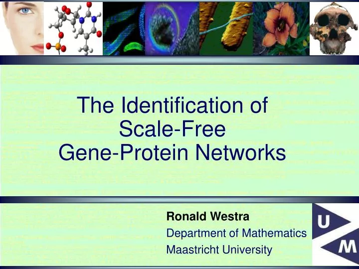
The Identification of Scale-Free Gene-Protein Networks. Ronald Westra Department of Mathematics Maastricht University. Items in this Presentation. 1. Biological background and problem formulation 2. Modeling of dynamic gene/proteins interactions 3. Scale-free network structures

E N D
The Identification of Scale-Free Gene-Protein Networks Ronald Westra Department of Mathematics Maastricht University
Items in this Presentation 1. Biological background and problem formulation 2. Modeling of dynamic gene/proteins interactions 3. Scale-free network structures 4. Reconstruction of scale-free gene/proteins networks 5. Conclusions
1. Biological background Do gene-protein networks exhibit characteristic architectural and structural properties that may act as a format for reconstruction? Some observations ...
Mycoplasma genitalium 500 nm 580 Kbp 477 genes 74% coding DNA Obligatory parasitic endosymbiont Mycoplasma genitalium Metabolic Network Degree distribution Horizontally log of degree (= number of connections), vertically log of number of genes with this degree Metabolic Network Nodes are genes, edges are gene co-expressions
Yeast Protein complex network and connected complexes in yeast S. cerevisiae, Gavin et al., Nature 2002. Cumulative degree distributions of Saccharomyces cerevisiae, Jeong et al, Nature 2001
Functional modules of the kinome network [Hee, Hak, 2004]
Degree distributions in human gene coexpression network. Coexpressed genes are linked for different values of the correlation r, King et al, Molecular Biology and Evolution, 2004
Statistical properties of the human gene coexpression network. • Node degree distribution. • Clustering coefficient plotted against the node degree • King et al, Molecular Biology and Evolution, 2004
Problem formulation • Objective: • * Are there distinctive architectural properties in gene-protein networks that facilitate their reconstruction from experimental data? (it helps if you know how it looks like) • Example: sparsity (Yeung et al. 2003, etc) • * Are there other special network properties that work similarly? Or even better?
2. Modeling Interactions between Genes and Proteins Prerequisite for the successful reconstruction of gene-protein networks is the way in which the dynamics of their interactions is modeled.
Components in Gene-Protein networks Genes: ON/OFF-switches (→ continuous) RNA&Proteins: vectors of information exchange between genes External inputs: interact with higher-order proteins
General state space dynamics The evolution of the n-dimensional state space vector x (gene expressions/protein densities) depend on p-dim inputs u, system parameters θ and Gaussian white noise ξ.
external inputs genes/proteins input-coupling interaction-coupling Example of an general dynamics network topology
Problems with modeling the general network dynamics • The general case is too complex • Strongly dependent on unknown microscopic details • Relevant parameters are unidentified and thus unknown • Therefore approximate interaction potentials and qualitative methods seem appropriate • Here some (of the many, many) practical approaches …
x : the vector (x1, x2,..., xn) where xi is the relative gene expression of gene ‘í’ u : the vector (u1, u2,..., up) where ui is the value of external input ‘í’ (e.g. a toxic agent) νξ(t) : white Gaussian noise 1. Linear stochastic state-space models FollowingP. D'Haeseleer, M. B. Eisen, S. Yeung, P. T. Spellman, and many others
2. Piecewise Linear Models FollowingMestl, Plahte, Omhold 1995 and others bilsum of step-functions s+,–
3. More complex non-linear interaction models Example: rational functions = quotient of polynomials: Example: Michaelis-Menten →
Objectives in reconstruction of (linear) networks Mathematical modelM: Experimental data D: Objective:Find the model parameters A and B such that the model M matches the data D.
Reconstruction of SPARSE LINEAR networks In most cases the mathematical complexities in finding a realistic network structure are too severe Therefore, some researchers have introduced new constraints that facilitate the computation The best example is SPARSITY in a LINEAR network :
Major Problem in reconstruction of sparse networks The system is severely under-constrained as there are typically far more model parameters A and B than there is experimental dataD. A useful trick is to assume that the system is heavilysparseandlinear [Yeung et al, Guthke et al, …] In that case the system can be: (i) decomposed row-for-row, and (ii) L1-regression can be employed
M: → D: Decoupling: → D z p Sparsity: L1-regression: →
Result: Above a minimum number Mmin of measurements and with a maximum number kC of non-zeros the reconstruction is perfect. Mmin is much smaller than in L2-regression, Mmin and kC depend on N.
3. Using special architectures of gene-protein networks So far we used the fact that biological information processing networks mostly exhibit only a few connections (=sparse) and only a few genes and proteins control a considerable amount of all others (=hierarchic) Other interesting properties of networks are also observed : regular, small world, scale free, exponential, apollonian, …
Network Architectures There is more internal structure in a gene-protein network which we can use to derive more powerful constraints, and the most interseting is the Scale-Free (SF) property
What is the Scale-free property? In a scale-free network the degree distribution follows a power law. The degree distribution is the fraction nSF(k) of nodes in the network having k connections to other nodes. In SF networks this goes (for large values of k) as: nSF(k) ~ k−γ where γ is a constant whose value is typically in the range 1<γ<3, although occasionally it may lie outside these bounds.
Why Scale-free? Scale-free networks are noteworthy because many empirically observed networks appear to be scale-free, including the world wide web, protein networks, citation networks, and social networks.
Cumulative degree distributions in the interaction network of genes and proteins in the metabolism of Saccharomyces cerevisiae [Jeong et al, Nature 2001]
Clustering of co-expression profiles using K-nearest neighbor algorithm • For each node (gene/protein) determine the K closest (= most similar) nodes • Two nodes are joined in the graph if they are in each others K-nearest neighbor set • Examine the resulting network graph – especially for SF-ness
Clustering of co-expression profiles using K-nearest neighbor algorithm Cumulative distribution F of degree distribition P:
Colon cancer data of Alon et al. PNAS 1999, Breast cancer data of Perou et al. PNAS 1999
Clustering of co-expression profiles using K-nearest neighbor algorithm Order parameter Λ: H. Agrawal, Physical Review letters, 2002
Colon cancer data of Alon et al. PNAS 1999, Breast cancer data of Perou et al. PNAS 1999 This closes the case for the biological relevance of scale-free networks …
CENTRAL THOUGHT Conjecture: Scalefree-ness in a (gene regulatory) network implies sparsity. SF is much stronger than sparsity … it also requires a specific distribution of connections in the network – and hence in the connectivity matrix, namely the SF powerlaw Not only a large number of zeros are required, they are also grouped in a special manner.
Relation between Scalefree and Sparse Define: sparsity = number of connections/ n(n-1)/2 For n=10,000 : gamma log(sparsity) 1 -1.5888 2 -6.9176 3 -9.5158 4 -10.7187 5 -11.6457
Reconstruction of scalefree networks For these reasons, the reconstruction of networks using the SF-property should be much more effective than from sparse networks
Requirements For the reconstruction of a scalefree (gene-protein) interaction system we need: 1. a suitable parametrised formal model 2. a method for optimising the scalefreeness of the system with respect to the model parameters for a given set of measurements (e.g. microarrays) We will visit these items in the following slides ...
4. Reconstruction of scalefree gene-protein networks Philosophy: The experimental data bounds the feasible parameter set A and B, and the scalefree-ness (SF) of A and B should be as high as possible consistent with the data D
Linear Model of gene-protein networks • For simplicity we assume a non-symmetric, and SF gene/protein network with a linear state space dynamics • Suppose we have a set of M observations of genome-wide expression profiles (e.g. microarrays)
Linearized form of a subsystem First order linear approximation of system separates state vector x and inputs u.
Experimental Data: Now, suppose that we have M data items (e.g. microarray measurements) we want to map to the network:
Data Match The relation between the desired patterns (state derivatives, states and inputs) defines constraints on the data matrices A and B, which have to be computed.
Data Match If you don’t like a continuous model just use a discrete model:
Scalefree-ness Now compute the observed degree-distribution in the system matrix M : DegDist(k,M) : the number of nodes with degree k As we are now dealing with a directed graph, there is a difference between in-coming and out-going connections. We will here consider only the out-degree. Note that hierarchy of the net relates to the in-degree.
Scalefree-ness The out-degree distribution Degree(k,C) of a connectivity matrix C is the sum of the k-th column: Degree(k,C) = Σm cmk = 1T.C Example: C = Degree(k,C) =
Scalefree-ness The degree is the basis for computing the degree distribution DegDist(k,C) of a connectivity matrix C. How can we determine the connectivity matrix for an arbitrary interaction matrix M like the matrices A and B in our linear model? Answer: we approximate the connectivity matrix of M to an accuracy ε as Cε(M), similar to the approximation δε(x) of the δ-function δ(x) in measure theory …