Download
1 / 32
320 likes | 445 Views
Adaptive Radio Interference Positioning System. Modeling and Optimizing Positional Accuracy based on Hyperbolic Geometry. Hao-ji Wu, Henry Chang, Bing You, Hao Chu , Polly Huang National Taiwan University. The Short Story. Improve accuracy of the RIP system (Vanderbilt U.)

E N D
Adaptive Radio Interference Positioning System Modeling and Optimizing Positional Accuracy based on Hyperbolic Geometry Hao-ji Wu, Henry Chang, Bing You, Hao Chu, Polly Huang National Taiwan University
The Short Story Improve accuracy of the RIP system (Vanderbilt U.) RIP: Radio interference positioning Improvement comes from our adaptive mechanism Model the error in the original RIP system From the error model, identify the controllable parameter (i.e., beacon node selection) Adapt based on the controllable parameter Implemented & evaluated in a real testbed Verified our error model is accurate Showed our accuracy improvement is real.
Motivation • Accuracy and precision are important performance goals in localization systems. • WiFi localization systems > 1 meter • Look for a localization system with sub-meter positional accuracy (ideally with long range and low cost) similar to WiFi. • Duplicate it and improve upon it. (about the same time last year.)
Radio Interference Positioning (RIP) System • Proposed by Vanderbilt University (Kusy et al) • Found it in Sensys 2005 • Recent papers: Sensys 2007, Mobisys 2007, IPSN 2006, etc. • High accuracy • Average accuracy 3 cm (Sensys’05) • Long sensing range • 160 meters (Sensys’05), few nodes can cover wide area • Low cost • Using standard sensor network nodes (Mica2), no additional specialized hardware • Amazing accuracy? • Mica2 node dimension (5.8 x 3.2 x 0.7) cm
Two starting questions Are the RIP system results reproducible? Can the RIP system be improved further? 6
Our Findings Are the RIP results reproducible? Reproduced results Average: 75 cm; 90%: 1.41 meters Experimental setup is slightly different form Vanderbilt U. 900 Mhz versus 433 Mhz (Vanderbilt U.) 3 cm is very ideal situation Can the RIP system be improved further? More room for improvement in our adaptation mechanism 7
Overview of RIP system Ranging Positioning • Two phases • In the ranging phase: two ranging rounds • In each ranging round, we need to select two beacon nodes(called sender-pair) • Target is a receiver • Another infrastructure node is a receiver • Why two beacon nodes? Anchor node (known location)
A, B are senders Transmit at two nearby frequency (900 MHz) Produce an interference wave with low-beat frequency envelop (350 Hz) C (target), D are receivers Each detects phase, and jointly the phase difference Map the phase difference to a distance difference | AC – BC | From Sensys 2005 (Kusy et al)
RIP ranging & positioning • Ranging_result = distance(T,sender1) – distance(T,sender2) = d1 – d2 • Each ranging result in a hyperbolic curve • Two ranging needed for positioning • Two sender-pairs selected in two ranging round are called Sender Pair Combination(SPC) sender1 sender2 sender1 d1 d2 d1 T d2 sender2
Modeling Position Error in RIP Ranging phase Imperfect measurements lead to ranging error, i.e., error in (d1 – d2) ~ 26 cm, more or less independent of distance to the beacon Ranging error leads to shift in the hyperbolic curve Positioning phase Compute intersection of two shifted hyperbolic curves (due to ranging errors) Ranging error may amplify the positioning error to different amounts Depend on the geometry layout between target and SPCs [an example] 11
How geometry layout affects positional error? • Two geometry layouts from two different SPC selections • With the same amount of range error, Layout (A) has a larger error than Layout (B), why? • Can you identify two geometric properties leading to the larger error in (A)? sender1 sender2 (A) (B) sender1 sender1 sender2 Errorrange T T T’ T’ sender2 sender1 sender2
Geometric property #1 • The position of T on the curve • Closer to the foci, smaller the error displacement from the curve, and smaller the error amplification sender1 sender2 Errorrange T T sender1 sender2
Geometric property #2 • Intersectional angle of hyperbolic curves • Shaper the intersectional angle, larger the error amplification T T T θ θ θ T’ T’ T’ θ= 90° θ= 60° θ= 30°
Geometric property #2 (cont.) • Intersectional angle of hyperbolic curves • (A) has sharper intersectional angle than (B) sender1 sender2 (A) (B) sender1 sender1 sender2 Errorrange θ θ T T T’ T’ sender2 sender1 sender2
Validation of Estimation Error Model Static RIP (6 anchor nodes, 10 meters radius) Blue line : target path Blue point : ground truth Red point : estimation position 17
Validation of Estimation Error Model Estimation error falls within 6 cm 90% of the time. 18
Adaptive RIP system • We have an accurate Estimation Error Model • Predict Errorpositionalusing specific SPC • We run Estimation Error Model for all SPC (exhaustive search), and find the SPC with minimum error
Evaluation of adaptive RIP system • Single-target positioning experiment • Multi-target positioning experiment A~F are anchor nodes Each grid is 1m2
Single-target positioning experiment Static RIP Adaptive RIP Blue line : target path Blue point : ground truth Red point : estimation position
Single-target positioning experiment walking repeatedly 5 times, around 50 samples
Multi-target positioning experiment • 6 targets • 1 moving (blue point) • 5 static (1~5 green points)
Conclusion • Error in RIP system is determined by geometric location of the target and beacons. • We created an Error Estimation Model • Estimate error given relative location of the target and SPCs. • Adaptive mechanism is built upon the error estimation model. • Find SPC with minimum error • Showed that Error Estimation Model is accurate. • Showed that Adaptive mechanism improves accuracy.
Flow of RIP system Sender1 Receiver1 Receiver1 Ranging Positioning Sender1 • Start RIP system • Select 2 anchor nodes as senders • Other anchor nodes become receiver • Ranging • If 1st ranging => goto 2 and do 2nd ranging else => goto 6 do positioning • Positioning • End 2nd ranging 1st ranging T Receiver2 Sender2 Receiver2 Sender2 Anchor node (known location)
Geometrical Derivation of Estimation Error Model • Steps: • Find TN (TM) • Find θ • Find PT geometrically mN • Known Variables: • Target location • SPC • Errorrange mM If we know TN, TM, θ, we can derivativePT geometrically
Original RIP system Anchor nodes are placed in known locations The positional error of RIP system is highly affected by targetlocations and the selection of beacon nodes Original RIP system is “static” The selection of beacon nodes is fixed, doesn’t change depend on target locations Beacon T Beacon 29
Our Contribution Design, implement and evaluate an adaptive RIP system Dynamically select beacon nodes based on target locations 30
How SPC selection affect positional error (cont.) Displacement of a hyperbolic curve Shortest distance from hyperbolic curve with error to target sender1 sender2 Errorrange T T sender1 sender2 31
PT is the estimation Errorpositional N is the projection point of T on H12 TN is the displacement of hyperbolic curvesH12 θ is the intersectional angle of hyperbolic curvesH12 and H34 Find TM (TN) and θ geometrically Find PT geometrically Map Geometry properties to estimation error model Errorrange 32