Download
1 / 16
160 likes | 174 Views
Geometric Objects and Transformations. Chun-Yuan Lin The contexts of this slide is similar to Chapter 5-Geometric Transformations. Scalar, Points and Vectors (1). Geometric Objects Scalar, points and vectors Coordinate-Free Geometry The Mathematical View-Vector and Affine Spaces.

E N D
Geometric Objects and Transformations Chun-Yuan Lin The contexts of this slide is similar to Chapter 5-Geometric Transformations CG
Scalar, Points and Vectors (1) • Geometric Objects • Scalar, points and vectors • Coordinate-Free Geometry • The Mathematical View-Vector and Affine Spaces CG
Scalar, Points and Vectors (2) • The Computer Science View • Abstract data types (ADT) • Geometric ADTs • Lines • Affine Sums • Convexity CG
Scalar, Points and Vectors (3) • Dot and Cross Products • Planes CG
Three-Dimensional Primitives • Three features characterize three-dimensional objects that fit with existing graphics hardware and software. • The objects are described by their surfaces and can be thought of as being hollow. • The objects can be specified through a set of vertices in three dimensions. • The objects either are composed of or can approximated by flat, convex polygons. CG
Coordinate Systems and Frames • Representation and N-tuples • Change of coordinate systems • Example Change of Representation • Homogeneous Coordinates • Example Change in Frames • Working with Representations CG
Frames in OpenGL • For most of geometric problems, we usually go from one frame to another by a sequence of geometric transformations such as rotations, translations and scales. CG
Modeling a Color Cube (1) • Modeling the faces • The cube is as simple a three-dimensional objects as we might expect to model and display. • There are several ways to model it. Example: GLfloat vertices[8][3]= {{}, {},{},{},{},{},{},{}}; • We can adopt a more object-orient form . typedef GLfloat point3[3]; point3 vertices[8]= {{}, {},{},{},{},{},{},{}}; CG
Modeling a Color Cube (2) • We can then use the list of points to specify the face of the cube. For one face: glBegin(GL_POLYGON); glVertex3fv (vertices[0]); glVertex3fv (vertices[3]); glVertex3fv (vertices[2]); glVertex3fv (vertices[1]); glEnd(); CG
Modeling a Color Cube (3) • Inward- and Outward-Pointing Faces • We call a face outward facing if the vertices are traversed in a counterclockwise order when the face is viewed from the outside. (right-hand rule) • Data structures for Object Representation glBegin(GL_POLYGON) glBegin(GL_QUADS) CG
Modeling a Color Cube (4) • Vertex list CG
Modeling a Color Cube (5) • The color cube • We assign a color for the face using the index of the first vertex. • Bilinear Interpolation CG
GLfloat vertices[8][3] = {{-1.0,-1.0,-1.0},{1.0,-1.0,-1.0}, {1.0,1.0,-1.0}, {-1.0,1.0,-1.0}, {-1.0,-1.0,1.0}, {1.0,-1.0,1.0}, {1.0,1.0,1.0}, {-1.0,1.0,1.0}}; GLfloat colors[8][3] = {{0.0,0.0,0.0},{1.0,0.0,0.0}, {1.0,1.0,0.0}, {0.0,1.0,0.0}, {0.0,0.0,1.0}, {1.0,0.0,1.0}, {1.0,1.0,1.0}, {0.0,1.0,1.0}}; void quad(int a, int b, int c, int d) { glBegin(GL_POLYGON); glColor3fv(colors[a]); glVertex3fv(vertices[a]); glColor3fv(colors[b]); glVertex3fv(vertices[b]); glColor3fv(colors[c]); glVertex3fv(vertices[c]); glColor3fv(colors[d]); glVertex3fv(vertices[d]); glEnd(); } void colorcube() { quad(0,3,2,1); quad (2,3,7,6); quad (0,4,7,3); quad (1,2,6,5); quad (4,5,6,7); quad(0,1,5,4); } CG
Modeling a Color Cube (6) • Vertex Arrays • Vertex arrays provide a method for encapsulating the information in the data structure such that we can draw polyhedral objects with only a few function calls. glEnableClientState(GL_COLOR_ARRAY); glEnableClientState(GL_VERTEX_ARRAY); glVertexPointer(3, GL_FLOAT,0,vertices); glColorPointer(3,GL_FLOAT,0, colors); Glubyte cubeIndices[24]={0,3,2,1,2,3,7,6,0,4,7,3,1,2,6,5,4,5,6,7,0,1,5,4}; CG
Modeling a Color Cube (7) • We can render the cube through use of the arrays. glDrawElements(GLenum type, GLsize n, GLenum format, void *pointer) example: for(i=0;i<6;i++) glDrawElements(GL_POLYGON, 4, GL_UNSIGNED BYTE, &cubeIndices[4*I]); Or glDrawElements(GL_QUADS, 24, GL_UNSIGNED BYTE, cubeIndices); CG
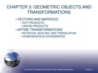
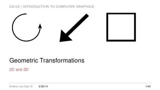
Affine Transformations Translation, Rotation and Scaling Transformations in Homogeneous Coordinates Concatenation of Transformations OpenGL Transformation Matrices CG