Download
1 / 46
460 likes | 606 Views
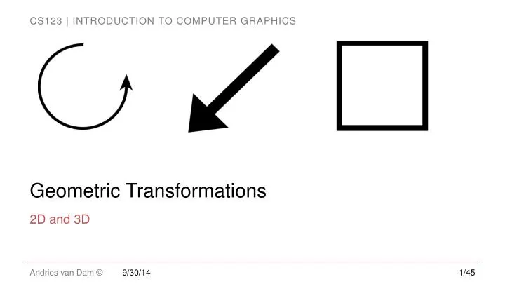
Geometric Transformations. 2D and 3D. How do we use Geometric Transformations? (1/2). Objects in a scene at the lowest level are a collection of vertices… These objects have location, orientation, size Correspond to transformations: Translation ( T ), Rotation ( R ), and Scaling ( S ).

E N D
Geometric Transformations 2D and 3D 9/30/14
How do we use Geometric Transformations? (1/2) • Objects in a scene at the lowest level are a collection of vertices… • These objects have location, orientation, size • Correspond to transformations: Translation (T), Rotation (R), and Scaling (S) 9/30/14
How do we use Geometric Transformations? (2/2) • A scene has a camera/view point from which the scene is viewed • The camera has some locationand some orientation in 3-space … • These correspond to Translation and Rotation transformations • Need other types of viewing transformations as well - learn about them shortly 9/30/14
Some Linear Algebra Concepts... • 3D coordinate geometry • Vectors in 2 space and 3 space • Dot product and cross product – definitions and uses • Vector and matrix notation and algebra • Identity matrix • Multiplicative associativity • E.g. A(BC) = (AB)C • Matrix transpose and inverse – definition, use, and calculation • Homogeneous coordinates (x, y, z, w) • You will need to understand these concepts! • Linear algebra help session notes: • http://cs.brown.edu/courses/cs123/resources/Linear_Algebra.pdf 9/30/14
Linear Transformations (1/3) • We represent vectors as bold-italic letters (v) and scalars as italic letters (c) • Any vector in the plane can be defined as the sum of two non-collinear basis vectors • Recall that a basis for a vector space is a set of vectors with the following properties: • The vectors in the set are linearly independent • Any vector in the vector space can be expressed as a linear combination of the basis vectors • Multiplying a vector by a scalar changes the vector’s magnitude b a v = a + b v 9/30/14
Linear Transformations (2/3) • Definition of a linear function f: • f(v+w) = f(v) + f(w) for all v and w in the domain of f • f(cv) = cf(v) for all scalars c and elements v in the domain • Example: f(x) = f(x1 , x2) := (3x1+2x2 , -3x1+4x2) • Now let v and w be two elements in the domain of f • f(v+w) = f(v1+w1 , v2+w2) • = (3(v1+w1)+2(v2+w2) , -3(v1+w1)+4(v2+w2)) • = (3v1+2v2, -3v1+4v2) + (3w1+2w2, -3w1+4w2) • = f(v) + f(w) • We can check the second property the same way • Both properties must be satisfied for the function f to be linear f(e2) e2 e1 f(e1) 9/30/14
Linear Transformations (3/3) • Graphical use: transformations of points around the origin (leaves the origin invariant) • These include Scaling and Rotations • Translation is not a linear function (moves the origin) • Any linear transformation of a point will result in another point in the same coordinate system, transformed about the origin • Aside: How do we know the origin is invariant from the definition of linearity? 9/30/14
Linear Transformations as Matrices (1/2) • Linear transformations can be represented as invertible (non-singular) matrices • Let’s start with 2D transformations. These can be represented by 2x2 matrices: • A transformation of an arbitrary column vector x = has the form: 9/30/14
Linear Transformations as Matrices (2/2) • Let e1 and e2be the standard basis vectors: • Now substitute each basis vector for x to get: • Notice that the columns of the matrix representation of our transformation matrix T are precisely T applied to e1 and e2: • This gives us a strategy for deriving transformation matrices! • We can derive the columns of a transformation matrix one by one by considering how our desired transformation affects each of the standard unit vectors. 9/30/14
Scaling in 2D (1/2) • Scale x by 3, y by 2 (Sx = 3, Sy = 2) • v = (original vertex); v’ = (new vertex) • v’ = Sv • Derive S by determining how e1 and e2 should be transformed • (scale in X by Sx) • (scale in Y by Sy) • Thus we obtain Side effect: House shifts position relative to origin 9/30/14
Scaling in 2D (2/2) • S is a diagonal matrix; we can quickly check using matrix multiplication that our derivation is correct: • S multiplies each coordinate of v by the appropriate scaling factor, as expected • In general, the ith entry of Dv, where D is diagonal, is (D[i,i] * v[i]) • Properties of scaling to look out for: • Does not preserve angles between lines in the plane (except when scaling is uniform, i.e. sx= sy) • If the object doesn’t start at the origin, scaling will move it closer to or farther from the origin (often not desired) 9/30/14
Rotation in 2D (1/2) • Rotate by θ about the origin • v’ = Sv, where • v = (original vertex) • v’ = (new vertex) • Derive Rθ by determining how e1and e2 should be transformed: • (first column of Rθ) • (second column of Rθ) 9/30/14
Rotation in 2D(2/2) • Let’s try matrix-vector multiplication • Rθ * v = • Other properties of rotation: • Preserves lengths in objects and angles between parts of objects (rigid-body rotation) • For objects not centered at the origin, an unwanted translation might be introduced (rotation is always about the origin) 9/30/14
What about translation? • Translation is not a linear transformation (the origin is not invariant) • Therefore, it can’t be represented as a 2x2 invertible matrix • Question: Is there another solution? • Answer: Yes, v’ = v + t, where t = • However, using vector addition is not consistent with our method of treating transformations as matrices • If we could treat all transformations in a consistent manner, i.e., with matrix representation, then could combine transformations by composing their matrices • Let’s try using a matrix again • How? Homogeneous Coordinates: add an additional dimension, the w-axis, and an extra coordinate, the w-component • Thus 2D -> 3D (effectively the hyperspace for embedding 2D space) 9/30/14
Homogeneous Coordinates (1/3) • Allow expression of all three 2D transformations as 3x3 matrices • We start with the point P2d on the xy plane and apply a mapping to bring it to the w-plane in the hyperspace • P2d(x,y) Ph(wx, wy, w), w≠0 • The resulting (x’,y’) coordinates in our new point Phare different from the original (x,y), since x’ = wx, y’ = wy • Ph(x’, y’, w), w ≠ 0 9/30/14
Homogeneous Coordinates (2/3) • Once we have this point, we can apply a homogenized version of our T, R and S transformation matrices (next slides) to get a new point in the hyperspace • Finally, we want to obtain the corresponding point in 2D-space, so perform the inverse of the previous mapping (divide all entries by w) • The vertex v = is now represented as • v = 9/30/14
Homogeneous Coordinates (3/3) • The transformations we use will always map points in the hyperplane defined by w = 1to other such points. (That way, we don’t have to divide by w to get our equivalent point in 2D) • In other words, we want our transformations T to map points v = to • points v’ = • How do we achieve this with the matrices we have already derived? • For linear transformations (i.e. scaling and rotation), embed the existing matrix in the upper-left of a new 3x3 matrix: 9/30/14
Back to Translation • Our translation matrix (T) can now be represented by embedding the translation vector in the right column: • To verify that this is the right matrix, multiply it by our homogenized point: • Coordinates have been translated, and v’ is still homogeneous 9/30/14
Transformations Homogenized • Let’s homogenize our all matrices! Doesn’t affect linearity of scaling and rotation • Our new transformation matrices look like this… • Note: These transformations are called affine transformations, which means they preserve ratios of distances between points on a straight line 9/30/14
Examples • Scaling: Scale by 15 in the x direction, 17 in the y • Rotation: Rotate by 123o • Translation: Translate by -16 in the x direction, +18 in the y 9/30/14
Before we continue! Vectors vs. Points • Up until now, we’ve only used the notion of a point in our 2D space • We now present a distinction between points and vectors • We used homogeneous coordinates to more conveniently represent translation; hence points are represented as (x, y, 1)T • A vector can be rotated/scaled, but not translated (can think of it as always starting at origin), so don’t use the homogeneous coordinate: (x, y, 0)T • That way, the translation matrix won’t have any affect on our vectors. • For now, let’s focus on just our points (typically vertices) 9/30/14
Inverses • When we want to undo a transformation, we’ll need to find the matrix’s inverse. • Thanks to homogenization, they are all invertible! 9/30/14
A moment of appreciation for linear algebra • The inverse of a rotation matrix M is just its transpose MT! That’s really convenient, so let’s understand how it works using orthonormal matrices • Take a rotation matrix M = [v1 v2 v3] (where each viis a vector) • First note some properties of M • The columns are orthogonal to each other: vi • vj = 0 (i ≠ j) • Columns have unit length: ||vi|| = 1 • Let’s see what multiplying MTand M produces: • Using the properties above, we see that this is the identity matrix, so MT = M-1 9/30/14
More with Homogeneous Coordinates • Some uses we’ll see later: • Placing sub-objects in parent’s coordinate system to construct hierarchical scene graph • Transforming primitives in their own coordinate systems • View volume normalization • Mapping arbitrary view volume into canonical view volume along z-axis • Parallel (orthographic, oblique) and perspective projections • Perspective transformation (turn viewing pyramid into a cuboid to turn perspective projection into parallel projection) after perspective foreshortening 9/30/14
Composition of Transformations (2D) (1/2) • We now have a number of tools at our disposal; we can combine them! • An object in a scene uses many transformations in sequence. How do we represent this in terms of functions? • Transformation is a function; by associativity, we can compose functions: • (f o g)( i ) • This is the same as first applying g, then applying f: • f( g( i ) ) • Consider our functionsf and g as matrices (M1and M2) and our input as a vector v • Our composition is equivalent to M1M2v 9/30/14
Composition of Transformations (2D) (2/2) • We can now form compositions of transformation matrices to form a more complex transformation • For example, TRSv, which scales a point, then rotates it, then translates it: • Note that we apply the matrices in sequence right to left. We can use associativity to compose them first; it is often useful to be able to apply a single matrix if, for example, we want to use it to transform many points at once. • Important: order matters! Matrix multiplication is NOT commutative. • Be sure to check out the Transformation Game at http://www.cs.brown.edu/exploratories/freeSoftware/repository/edu/brown/cs/exploratories/applets/transformationGame/transformation_game_guide.html • Let’s see an example… 9/30/14
6 6 5 5 4 4 Y 3 3 2 2 1 1 0 0 1 1 2 2 3 3 4 4 5 5 6 6 7 7 8 8 9 9 10 10 X Not commutative Translate by x = 6, y = 0, then rotate by 45o Rotate by 45o, then translate by x = 6, y = 0 9/30/14
Composition (an example) (2D) (1/2) -Rotate 90o -Uniform scale 4x -Both around object’s center, not the origin • Start: Goal: • Important concept: make the problem simpler • Translate object to origin first, scale, rotate, and translate back: • Apply to all vertices 9/30/14
Composition (an example) (2D) (2/2) • T-1RST • But what if we mixed up the order? Let’s try RT-1ST: • Oops! We scaled properly, but when we rotated the object, it’s center was not at the origin, so its position was shifted. Order matters! 9/30/14
6 5 Y 4 3 2 1 0 1 2 3 4 5 6 7 8 9 10 X Aside: Skewing/shearing • “Skew” an object to the side, like shearing a card deck by displacing each card relative to the previous one • What physical situations mirror this behavior? • Squares become parallelograms; x-coordinates skew to right, y stays the same • Notice that the base of the house (at y = 1) remains horizontal but shifts right. Why? 2D non-homogeneous 2D homogeneous 9/30/14
Inverses Revisited • What is the inverse of a sequence of transformations? • (M1M2…Mn)-1 = Mn-1Mn-1-1…M1-1 • Inverse of a sequence of transformations is the composition of the inverses of each transformation in reverse order (why?) • Say we want to do the opposite transformation of the example on slide 27. What will our sequence look like? • (T-1RST)-1 = T-1S-1R-1T • We still translate to the origin first, then translate back at the end! 9/30/14
Aside: Windowing Transformations (CG terminology) • Windowing transformation maps contents of 2D clip rectangle (“window”) to a “viewport” rectangle on the screen, e.g., interior canvas (“client area”) of a window manager’s window; also called window-to-viewport transformation • Sends rectangle with bounding coordinates (u1 , vi), (u2 , v2) to (x1 , y1), (x2 , y2) • The transformation matrix here is: 9/30/14
Aside: Transforming Coordinate Axes • We understand linear transformations as changing the position of vertices relative to the standard axes • Can also think of transforming the coordinate axes themselves • Just as in matrix composition, be careful of which order you modify your coordinate system Translation Rotation Scaling 9/30/14
Dimension++ (3D!) • How should we treat geometric transformations in 3D? • Just add one more coordinate/axis! • A point is represented as • A matrix for a linear transformation T can be represented as • where e3 is the standard basis vector along the z-axis, • But remember to use homogeneous coordinates! Embed scale and rotation matrices as upper left submatrices and translation vectors as upper right subvectors of the right column 9/30/14
Transformations in 3D 9/30/14
Rodrigues’s Formula… • Rotation by angle θ around vector u= [uxuyuz]T • Note: this is an arbitrary unit vector u in xyz-space • Here’s a not so friendly rotation matrix • This is called the coordinate form of Rodrigues’s formula • Let’s try a different approach… 9/30/14
Rotating axis by axis (1/2) • Every rotation can be represented as the composition of 3 different angles of counter-clockwise rotation around 3 axes, namely • x axis in the yz plane by ψ; yaxis in the xz plane by θ; zaxis in the xy plane by ϕ • Also known as Euler angles, make problem of rotation much easier • Note these differ only in how the 3x3 submatrix is embedded in the homogeneous matrix, but the row-column order is different for Rzx • You can compose these matrices to form a composite rotation matrix 9/30/14
y Rotating axis by axis (2/2) θ u • It would still be difficult to find the 3 angles to • rotate by, given arbitrary axis u and specified angle ψ • Solution? Make the problem easier by • mapping u to one of the principal axes • Step 1: Find a θto rotate around y axis • to put u in the xy plane • Step 2: Then find a ϕ to rotate around • the z axis to align u with thexaxis • Now that uis in a convenient alignment, we can do our transformation rotation for vertex v: • Step 3: Rotate v by ψ around x axis (which is coincident with u axis) • Step 4: Finally, undo the alignment rotations (inverse). • The only rotation we’ve preserved is the one around axis uby ψ, which was our goal • Rotation matrix: M = Rzx-1(θ)Rxy-1(ϕ)Ryz(ψ)Rxy(ϕ)Rzx(θ) v v ψ u x v ϕ z 9/30/14
Inverses and Composition in 3D! • Inverses are once again parallel to their 2D versions… • Composition works exactly the same way… 9/30/14
Example in 3D! • Let’s take some 3D object, say a cube centered at (2,2,2) • Rotate in object’s space by 30o around x axis, 60o around y, and 90o around z • Scale in object space by 1 in the x, 2 in the y, 3 in the z • Translate by (2,2,4) in world space • Transformation sequence: TT0-1SxyRxyRzxRyzTo, where T0 translates to (0,0): T T0-1SxyRxyRzxRyz T0 9/30/14
Scene Graph ROBOT upper body lower body base stanchion head trunk arm Transformations and the scene graph (1/5) • Objects are typically composites: • 3D scenes are often stored in a directed acyclic graph (DAG) called a scene graph • WPF (Windows Presentation Foundation) • Open Scene Graph (used in the Cave) • X3D ™ (VRML ™ was a precursor to X3D) • most game engines • Typical scene graph format: • objects (cubes, sphere, cone, polyhedra etc.): • stored as nodes (default: unit size at origin) • attributes (color, texture map, etc.): stored as separate nodes • Transformations: also nodes arm Example scenegraph from a game engine 9/30/14
Transformations and the scene graph (2/5) • For your assignments use simplified format: • Attributes stored as a components of each object node (no separate attribute node) • A transform node affects its subtree • Only leaf nodes are graphical objects. • All internal nodes that are not transform nodes are object group nodes 9/30/14
Transformations and the scene graph (3/5) • Step 1: Various transformations are applied to each of the leaves (object primitives—head, base, etc.) • Step 2: Transformations are then applied to groups of objects (form upper and lower body, etc…) This format means that instead of designing new primitives for every single shape we need, we can just apply transformations to a smaller set of primitives to form complex composite 3D shapes. Represents a transformation Together the above hierarchy of transformations forms the “robot” scene as a whole 9/30/14
Transformations and the scene graph (4/5) • A cumulative transformation matrix (CTM) builds as you move up the tree. • Note that higher level transformation matrices are appended to the front of the sequence • Example: • For object 1 (o1), CTM = M1 • For o2, CTM = M2M3 • For o3, CTM = M2M4M5 • For a vertex v in o3, position in world coordinate system is CTMv = (M2M4M5) v M1 M2 M3 M4 M5 object nodes (geometry) transformation nodes group nodes 9/30/14
group3 root group1 obj4 obj3 obj1 group3 group2 obj2 group3 Transformations and the scene graph (5/5) • You can easily reuse groups of objects (sub-trees in the scene graph) if they have been defined already • This might occur if you have multiple similar components to your scene. For example, the robot’s 2 arms • Here, group 3 has been used twice. • Transformations defined within group 3 itself do not change; there are different CTMs for each use of group 3 as a whole • T0T1 vs. T0T2T4 9/30/14
Further Reading • More information can be found in the textbook • Read Chapters 10 and 11 for more detail and advanced topics on transformations • Chapter 7 discusses the 2D/3D coordinate space geometry • Chapter 12 goes into more detail about some of the linear algebra involved in graphics 9/30/14