Download

1 / 109
1.1k likes | 1.32k Views
Chapter 5: Physical Layer. Outline. Basic Components Source Encoding The Efficiency of a Source Encode Pulse Code Modulation and Delta Modulation Channel Encoding Types of Channels Information Transmission over a Channel Error Recognition and Correction Modulation Modulation Types

E N D
Outline • Basic Components • Source Encoding • The Efficiency of a Source Encode • Pulse Code Modulation and Delta Modulation • Channel Encoding • Types of Channels • Information Transmission over a Channel • Error Recognition and Correction • Modulation • Modulation Types • Quadratic Amplitude Modulation • Summary • Signal Propagation
Physical Layer • One of the desirable aspects of WSNs is their ability to communicate over a wireless link, so • mobile applications can be supported • flexible deployment of nodes is possible • the nodes can be placed in areas that are inaccessible to wired nodes • Once the deployment is carried out, it is possible to • rearrange node placement - optimal coverage and connectivity • the rearrangement can be made without disrupting the normal operation
Physical Layer • Some formidable challenges: • limited bandwidth • limited transmission range • poor packet delivery performance because of interference, attenuation, and multi-path scattering • therefore, it is vital to understand their properties and some of the mitigation strategies • this chapter provides a fundamental introduction to point-to-point wireless digital communication
Outline Basic Components Source Encoding The Efficiency of a Source Encode Pulse Code Modulation and Delta Modulation Channel Encoding Types of Channels Information Transmission over a Channel Error Recognition and Correction Modulation Modulation Types Quadratic Amplitude Modulation Summary Signal Propagation
Basic Components • The basic components of a digital communication system: • transmitter • channel • receiver • Here, we are interested in short range communication- because nodes are placed close to each other
Basic Components Figure 5.1 provides a block diagram of a digital communication system
Basic Components • The communication source represents one or more sensors and producesa message signal- an analog signal • the signal is a baseband signal having dominant frequency components near zero • the message signal has to be converted to a discrete signal (discrete both in time and amplitude) • The conversion requires sampling the signal at least atNyquist rate- no information will be lost • the Nyquist rate sets a lower bound on the sampling frequency • hence, the minimum sampling rate should be twice the bandwidth of the signal
Basic Components • Source encoding: the discrete signal is converted to a binary stream after sampling • An efficient source-coding technique can satisfy the channel’s bandwidth and signal power requirements • by defining a probability model of the information source • channel encoding- make the transmitted signal robust to noise and interference • transmit symbols from a predetermined codebook • transmit redundant symbols • Modulation- the baseband signal is transformed into a bandpass signal • main reason is to transmit and receive signals with short antennas
Basic Components • Finally, the modulatedsignalhas to beamplified and the electricalenergyis convertedintoelectromagneticenergyby the transmitter’s antenna • The signal is propagated over a wireless link to the desired destination • The receiver block carries out the reverse process to retrieve the message signal from the electromagnetic waves • the receiver antenna inducesavoltagethat is similar to the modulated signal
Basic Components • The magnitude and shape of the signal are changed because of losses and interferences • The signal has to pass through a series ofamplificationand filteringprocesses • It is then transformed back to a baseband signal through the process of demodulationand detection • Finally, the baseband signal undergoesa pulse-shaping processandtwostages of decoding(channel and source) • extract the sequence of symbols - the original analog signal (the message)
Outline Basic Components Source Encoding The Efficiency of a Source Encode Pulse Code Modulation and Delta Modulation Channel Encoding Types of Channels Information Transmission over a Channel Error Recognition and Correction Modulation Modulation Types Quadratic Amplitude Modulation Summary Signal Propagation
Source Encoding • A source encoder transforms an analog signalinto adigital sequence • The process consists of: sampling, quantizing, encoding • Suppose a sensor produces an analog signal s(t) • s(t)will be sampled and quantized by the analog-to-digital converter (ADC) that has a resolution ofQdistinct values • as a result, a sequence of samples, S = (s[1], s[2], ..., s[n])are produced • the difference between the sampled s[j]and its corresponding analog value at timetjis the quantization error • as the signal varies over time, the quantization error also varies and can be modeled as a random variable with a probability density function, Ps (t)
Source Encoding • The aim of the source encoder is to map each quantized element, s[j]into a corresponding binary symbol of lengthrfrom a codebook, C • Block code: if all the binary symbols in the codebook are of equal length • Often, the symbol length and the sampling rate are not uniform • It is customary to assign: • short-sized symbols and high sampling rates to the most probable sample values • long-sized symbols and low sampling rates to less probable sample values
Source Encoding Figure 5.2 illustrates the input – output relationship of a source encoder
Source Encoding • A codebook, C, can be uniquely decoded, if each sequence of symbols, (C(1), C(2), ...)can be mapped back to a corresponding value in S = (s[1], s[2], ..., s[n]) • A binary codebook has to satisfy Equation (5.1) to be uniquely decoded • where u is the size of the codebook • li is the size of the codeword C(i) Equation (5.1)
Source Encoding • A codebook can be instantaneously decoded • if each symbol sequence can be extracted (decoded) from a stream of symbols without taking into consideration previously decoded symbols • This will be possible • iff there does not exist a symbol in the codebook, such that the symbol a = (a1, a2, ..., am)is not a prefix of the symbol b = (b1, b2, ..., bn ), where m < nand ai= bi , ∀i = 1, 2, ...,mwithin the same codebook
Source Encoding Table 5.1Source-encoding techniques
Outline Basic Components Source Encoding The Efficiency of a Source Encode Pulse Code Modulation and Delta Modulation Channel Encoding Types of Channels Information Transmission over a Channel Error Recognition and Correction Modulation Modulation Types Quadratic Amplitude Modulation Summary Signal Propagation
The Efficiency of a Source Encoder • Quantity that expresses the average length • Sampled analog signal: L(C) = E [li(C)] • Suppose the probability of a q-ary source • i.e., it has qdistinct symbols • producing the symbol siis Piand the symbol Ciin a codebook is used to encode si • the expected length of the codebook is given by: Equation (5.2)
The Efficiency of a Source Encode • To express efficiency in terms of the information entropy or Shannon’s entropy • defined as the minimum message length necessary to communicate information • related to the uncertainty associated with the information • if the symbol sican be expressed by a binary symbol of nbits, the information content of siis: • the entropy (in bits) of a q-ary memoryless source encoder is expressed as: Equation (5.3) Equation (5.4)
The Efficiency of a Source Encode • The efficiency of a source encoder in terms of entropy reveals the unnecessary redundancy in the encoding process. This can be expressed by: • The redundancy of the encoder is: Equation (5.5) Equation (5.6)
Example Figure 5.3 An analog signal with four possible values
Example • In Figure5.3, it is quantized into four distinct values, 0, 1, 2, 3 • some values (2) occur more frequently than others (0 and 3) • if the probability of occurrence of these values is • P(0) = 0.05, P(1) = 0.2, P(2) = 0.7, P(3) = 0.05, then, • it is possible to compute the efficiency of two of the codebooks given in Table 5.1, namelyC2and C3 • for P1 = 0.05, log2( ) = 4.3. Becauselihas to be a whole number and there should be no loss of information, l1 must be 5. Likewise, l2 = 3; l3 = 1; and l4 = 5. Hence: Equation (5.7)
Example • Using Equation (5.4), the entropy of C2 is calculated as: • Therefore, the encoding efficiency of the codebook, C2(see Table 5.2) is: • The redundancy in C2 is: • in terms of energy efficiency, this implies that 30% of the transmitted bits are unnecessarily redundant, because C2 is not compact enough Equation (5.8) Equation (5.9) Equation (5.10)
Example Table 5.2 Description of the compactness of C2 Table 5.3 Description of the compactness of C3
Example • In the same way ljis computed forC2, the expected symbol length (in bits) for C3 (see Table 5.3) is given as: • Because the probabilities of the symbols are unchanged, entropy also remains unchanged. The encoding efficiency of C3 is therefore: • The redundancy, rdd, in C3 is: Equation (5.11) Equation (5.12) Equation (5.13)
Outline Basic Components Source Encoding The Efficiency of a Source Encode Pulse Code Modulation and Delta Modulation Channel Encoding Types of Channels Information Transmission over a Channel Error Recognition and Correction Modulation Modulation Types Quadratic Amplitude Modulation Summary Signal Propagation
Pulse Code Modulation and Delta Modulation • PCM and DM are the two predominantly employed source encoding techniques • In digital pulse code modulation • the signal is quantized first • each sample is represented by a binary word from a finite set of words • The resolution of a PCM technique and the source encoder bit rate are determined by • the size of the individual words • the number of words in the set
Pulse Code Modulation and Delta Modulation • In PCM, information is conveyed in the presence or absence of pulses • greatly enhances the transmission and regeneration of binary words • the associated cost with this form of source encoding is • the quantization error, the energy and bandwidth required to transmit the multiple bits for each sampled output • Figure 5.4 illustrates a PCM technique that uses two bits to encode a single sample • four distinct levels are permissible during sampling
Pulse Code Modulation and Delta Modulation Figure 5.4 A PCM based source encoding
Pulse Code Modulation and Delta Modulation • Delta modulation is a digital pulse modulation technique • it has found widespread acceptance in low bit rate digital systems • it is a differential encoder and transmits bits of information • the information describes the difference between successive signal values, as opposed to the actual values of a time-series sequence • the difference signal, Vd(t), is produced by first estimating the signal’s magnitude based on previous samples (Vi (t0)) and comparing this value with the actual input signal, Vin(t0)
Pulse Code Modulation and Delta Modulation • The polarity of the difference value indicates the polarity of the pulse transmitted • The difference signal is a measure of the slopeof the signal • first, sampling the analog signal • then, varying the amplitude, width, or the position of the digital signal in accordance with the amplitude of the sampled signal • Figure 5.5 illustrates delta modulation
Pulse Code Modulation and Delta Modulation Figure 5.5 Delta encoding
Outline Basic Components Source Encoding The Efficiency of a Source Encode Pulse Code Modulation and Delta Modulation Channel Encoding Types of Channels Information Transmission over a Channel Error Recognition and Correction Modulation Modulation Types Quadratic Amplitude Modulation Summary Signal Propagation
Channel Encoding • The main purpose is • to produce a sequence of data that is robust to noise • to provide error detection • to forward error correction mechanisms • The physical channel sets limits to • the magnitude • the rate of signal transmission • Figure 5.6 illustrates these restrictions
Channel Encoding Figure 5.6 Stochastic model of a channel
Channel Encoding • According to the Shannon – Hartley theorem, the capacity of a channel to transmit a message without an error is given as: • where C is the channel capacity in bits per second • Bis the bandwidth of the channel in hertz • Sis the average signal power over the entire bandwidth, measured in watts • Nis the average noise power over the entire bandwidth, measured in watts • Equation (5.14) states that for data to be transmitted free of errors, its transmission rate should be below the channel’s capacity • It also indicates how the signal-to-noise ratio (SNR) can improve the channel’s capacity Equation (5.14)
Channel Encoding • The equation reveals two independent reasons why errors can be introduced during transmission: • information will be lost if the message is transmitted at a rate higher than the channel’s capacity - equivocation(subtractive error) • information will be lost because of noise, which adds irrelevant information into the signal • A stochastic model of the channel helps to quantify the impact of these two sources of errors
Channel Encoding • Suppose an input sequence of data xlthat can havejdistinct values, xl∈ X = (x1, x2, ..., xj ), is transmitted through a physical channel • Let P(xl)denote P(X = xl) • The channel’s output can be decoded with a k-valued alphabet to produce ym∈ Y = (y1, y2, ..., yk) • Let P(ym)denotes P(Y = ym) • At timeti, the channel generates an output symbol yifor an input symbol xi
Channel Encoding • Assuming that the channel distorts the transmitted data, it is possible to model distortion as a stochastic process: where, l = 1, 2, ..., jand m = 1, 2, ..., k • In the subsequent analysis of the stochastic characteristic of the channel, the following assumptions hold: • the channel is discrete, namely, Xand Yhave finite sets of symbols • the channel is stationary, namely, P(ym|xl),are independent of the time instance, I • the channel is memoryless, namely, P(ym|xl),are independent of previous inputs and outputs Equation (5.15)
Channel Encoding • One way of describing transmission distortion is by using a channel matrix, PC Equation (5.16) where Equation (5.17) Moreover: Equation (5.18) Or, more generally: Equation (5.19) where both and are row matrices
Outline Basic Components Source Encoding The Efficiency of a Source Encode Pulse Code Modulation and Delta Modulation Channel Encoding Types of Channels Information Transmission over a Channel Error Recognition and Correction Modulation Modulation Types Quadratic Amplitude Modulation Summary Signal Propagation
Types of Channels • Binary Symmetric Channel • a channel model • bits of information (0 and 1) can be transmitted through it • the channel transmits a bit of information • correctly (regardless of whether information is 0 or 1) with a probability p • incorrectly (by flipping 1 to 0 and 0 to 1) with a probability 1 − p • the channel matrix of a binary symmetric channel: Equation (5.20) Equation (5.21) Equation (5.22)
Types of Channels • Binary Symmetric Channel Figure 5.7 A binary symmetric channel model
Types of Channels • Binary Erasure Channel • in a BEC, there is no guarantee that the transmitted bit of information can be received at all (correctly or otherwise) • a binary input - a ternary output channel • the probability of erasure ispand the probability that the information is correctly received is 1 − p • the probability of error is zero • a bit of information • either transmitted successfully with P(1|1) = P(0|0) = 1 − p • or erased altogether by the channel with a probability of p • the probability that 0 is received by transmitting 1 or vice versa is 0 Equation (5.23)
Types of Channels • Binary Erasure Channel Figure 5.8 A stochastic model of a binary erasure channel
Outline Basic Components Source Encoding The Efficiency of a Source Encode Pulse Code Modulation and Delta Modulation Channel Encoding Types of Channels Information Transmission over a Channel Error Recognition and Correction Modulation Modulation Types Quadratic Amplitude Modulation Summary Signal Propagation
Information Transmission over a Channel • Given the input message, , the channel matrix, [PC] • The output message, describe • the impact of irrelevance and equivocation • the percentage of information be transmitted over the channel without an error ---- transinformation or mutual information • Irrelevance • the content of information that can be introduced into the channel due to noise is described as the conditional information content, I (y|x) • the information content of ythat can be observed provided that xis known. The conditional entropy is given as: Equation (5.24)
Information Transmission over a Channel • P(y|x)can be known from the channel matrix [PC]. The average conditional entropy over all input message symbols, x∈X, is given by: • which is also equal to: • from Baye’s law, it is clear that: • according to Equation (5.26), a good channel encoder is one that reduces the irrelevance entropy Equation (5.25) Equation (5.26) Equation (5.27)