Download
1 / 40
400 likes | 421 Views
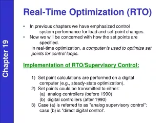
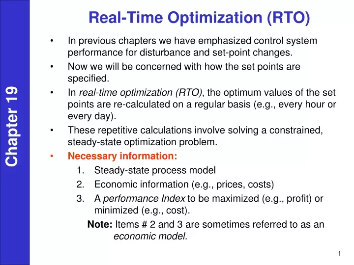
Real-Time Optimization (RTO) In previous chapters we have emphasized control system performance for disturbance and set-point changes. Now we will be concerned with how the set points are specified.

E N D
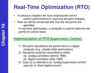
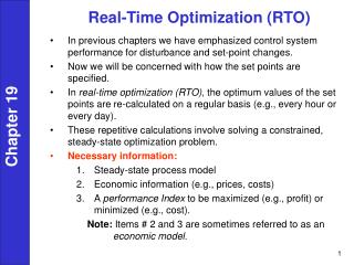
Real-Time Optimization (RTO) • In previous chapters we have emphasized control system performance for disturbance and set-point changes. • Now we will be concerned with how the set points are specified. • In real-time optimization (RTO), the optimum values of the set points are re-calculated on a regular basis (e.g., every hour or every day). • These repetitive calculations involve solving a constrained, steady-state optimization problem. • Necessary information: • Steady-state process model • Economic information (e.g., prices, costs) • A performance Index to be maximized (e.g., profit) or minimized (e.g., cost). Note: Items # 2 and 3 are sometimes referred to as an economic model. Chapter 19
Process Operating Situations That Are Relevant to Maximizing Operating Profits Include: • Sales limited by production. • Sales limited by market. • Large throughput. • High raw material or energy consumption. • Product quality better than specification. • Losses of valuable or hazardous components through waste streams. Chapter 19
Common Types of Optimization Problems • 1. Operating Conditions • Distillation column reflux ratio • Reactor temperature • 2. Allocation • Fuel use • Feedstock selection • 3. Scheduling • Cleaning (e.g., heat exchangers) • Replacing catalysts • Batch processes Chapter 19 3
BASIC REQUIREMENTS IN REAL-TIME OPTIMIZATION Objective Function: Chapter 19 • Both the operating and economic models typically will include constraints on: • Operating Conditions • Feed and Production Rates • Storage and Warehousing Capacities • Product Impurities
The Interaction Between Set-point Optimization and Process Control • Example: Reduce Process Variability • Excursions in chemical composition => off-spec products and a need for larger storage capacities. • Reduction in variability allows set points to be moved closer to a limiting constraint, e.g., product quality. Chapter 19
The Formulation and Solution of RTO Problems • Theeconomic model: An objective function to be maximized or minimized, that includes costs and product values. • The operating model: A steady-state process model and constraints on the process variables. Chapter 19
The Formulation and Solution of RTO Problems Table 19.1 Alternative Operating Objectives for a Fluidized Catalytic Cracker • Maximize gasoline yield subject to a specified feed rate. • Minimize feed rate subject to required gasoline production. • Maximize conversion to light products subject to load and • compressor/regenerator constraints. • Optimize yields subject to fixed feed conditions. • Maximize gasoline production with specified cycle oil • production. • Maximize feed with fixed product distribution. • Maximize FCC gasoline plus olefins for alkylate. Chapter 19
Selection of Processes for RTO • Sources of Information for the Analysis: • 1. Profit and loss statements for the plant • Sales, prices • Manufacturing costs etc. • 2. Operating records • Material and energy balances • Unit efficiencies, production rates, etc. • Categories of Interest: • 1. Sales limited by production • Increases in throughput desirable • Incentives for improved operating conditions and schedules. • 2. Sales limited by market • Seek improvements in efficiency. • Example: Reduction in manufacturing costs (utilities, feedstocks) • 3. Large throughput units • Small savings in production costs per unit are greatly magnified. Chapter 19 10
The Formulation and Solution of RTO Problems • Step 1. Identify the process variables. • Step 2. Select the objective function. • Step 3. Develop the process model and constraints. • Step 4. Simplify the model and objective function. • Step 5. Compute the optimum. • Step 6. Perform sensitivity studies. Chapter 19 Example 19.1 11
Chapter 19 UNCONSTRAINED OPTIMIZATION • The simplest type of problem • No inequality constraints • An equality constraint can be eliminated by variable substitution in the objective function.
Single Variable Optimization • A single independent variable maximizes (or minimizes) an objective function. • Examples: 1. Optimize the reflux ratio in a distillation column 2. Optimize the air/fuel ratio in a furnace. • Typical Assumption: The objective function f (x) is unimodal with respect to x over the region of the search. • Unimodal Function: For a maximization (or minimization) problem, there is only a single maximum (or minimum) in the search region. Chapter 19
Different Types of Objective Functions Chapter 19 15
One Dimensional Search Techniques • Selection of a method involves a trade-off between the number of objective function evaluations (computer time) and complexity. • 1. "Brute Force" Approach • Small grid spacing (x) and evaluate f(x) at each grid point can get close to the optimum but very inefficient. • 2. Newton’s Method Chapter 19 16
3. Quadratic Polynomial fitting technique • Fit a quadratic polynomial, f (x) = a0+a1x+a2x2, to three data points in the interval of uncertainty. • Denote the three points by xa, xb, and xc ,andthe corresponding values of the function as fa, fb, and fc. • Find the optimum value of x for this polynomial: Chapter 19 • Evaluate f (x*) and discard the x value that has the worst value of the objective function. (i.e., discard either xa, xb, or xc ). • Choose x* to serve as the new, third point. • Repeat Steps 1 to 5 until no further improvement in f (x*) occurs. 17
Equal Interval Search: Consider two cases Chapter 19 Case 1: The maximum lies in (x2, b). Case 2: The maximum lies in (x1, x3).
Multivariable Unconstrained Optimization • Computational efficiency is important when N is large. • "Brute force" techniques are not practical for problems with • more than 3 or 4 variables to be optimized. • Typical Approach: Reduce the multivariable optimization problem to a series of one dimensional problems: • (1) From a given starting point, specify a search direction. • (2) Find the optimum along the search direction, i.e., a • one-dimensional search. • (3) Determine a new search direction. • (4) Repeat steps (2) and (3) until the optimum is located • Two general categories for MV optimization techniques: • (1) Methods requiring derivatives of the objective function. • (2) Methods that do not require derivatives. Chapter 19 19
Constrained Optimization Problems • Optimization problems commonly involve equality and inequality constraints. • Nonlinear Programming (NLP) Problems: • a. Involve nonlinear objective function (and possible nonlinear constraints). • b. Efficient off-line optimization methods are available (e.g., conjugate gradient, variable metric). • c. On-line use? May be limited by computer execution time and storage requirements. • Quadratic Programming (QP) Problems: • a. Quadratic objective function plus linear equality and inequality constraints. • b. Computationally efficient methods are available. • Linear Programming (QP) Problems: • a. Both the objective function and constraints are linear. • b. Solutions are highly structured and can be rapidly obtained. Chapter 19 20
LP Problems (continued) • Most LP applications involve more than two variables and can involve 1000s of variables. • So we need a more general computational approach, based on the Simplex method. • There are many variations of the Simplex method. • One that is readily available is the Excel Solver. • Recall the basic features of LP problems: • Linear objective function • Linear equality/inequality constraints Chapter 19 21
Linear Programming (LP) • Has gained widespread industrial acceptance for on-line • optimization, blending etc. • Linear constraints can arise due to: • 1. Production limitation: e.g. equipment limitations, storage • limits, market constraints. • 2. Raw material limitation • 3. Safety restrictions: e.g. allowable operating ranges for • temperature and pressures. • 4. Physical property specifications: e.g. product quality • constraints when a blend property can be calculated as • an average of pure component properties: Chapter 19 22
5. Material and Energy Balances • - Tend to yield equality constraints. • - Constraints can change frequently, e.g. daily or hourly. • Effect of Inequality Constraints • - Consider the linear and quadratic objective functions on • the next page. • - Note that for the LP problem, the optimum must lie on one • or more constraints. • Solution of LP Problems • - Simplex Method • - Examine only constraint boundaries • - Very efficient, even for large problems Chapter 19 23
LinearProgramming Concepts • For a linear process model, y=Ku (19-18) Chapter 19
Chapter 19 25
Chapter 19 26
Chapter 19 27
Chapter 19 28
Chapter 19 29
Chapter 19 30
Chapter 19 31
Chapter 19 32
Chapter 19 33
Chapter 19 34
Chapter 19 35
Chapter 19 36
QUADRATIC AND NONLINEAR PROGRAMMING • The most general optimization problem occurs when both the objective function and constraints are nonlinear, a case referred to as nonlinear programming (NLP). • The leading constrained optimization methods include: • Quadratic programming • Generalized reduced gradient • Successive quadratic programming (SQP) • Successive linear programming (SLP) Chapter 19
Quadratic Programming • A quadratic programming problem minimizes a quadratic function of n variables subject to m linear inequality or equality constraints. • In compact notation, the quadratic programming problem is Chapter 19 where c is a vector (n x 1), A is an m x n matrix, and Q is a symmetric n x n matrix.
Nonlinear Programming • Constrained optimum: The optimum value of the profit is obtained • whenx=xa. Implementation of an active constraint is straight- • forward; for example, it is easy to keep a valve closed. • Unconstrained flat optimum: In this case the profit is insensitive • to the value of x, and small process changes or disturbances do not affect profitability very much. • Unconstrained sharp optimum: A more difficult problem for • implementation occurs when the profit is sensitive to the value of x. • If possible, we may want to select a different input variable for which the corresponding optimum is flatter so that the operating range can be wider. Chapter 19
Nonlinear Programming (NLP) Example - nonlinear objective function - nonlinear constraints Chapter 19 40