Download
1 / 121
1.25k likes | 1.34k Views
Two-Dimensional Inviscid Incompressible Fluid Flow. SOLO HERMELIN. Updated: 2.03.07 10.05.13. SOLO. 2-D Inviscid Incompressible Flow. TABLE OF CONTENT. Laplace’s Homogeneous Differential Equation. SOLO. 3-D Flow. Flow Description.

E N D
Two-Dimensional Inviscid Incompressible Fluid Flow SOLO HERMELIN Updated: 2.03.07 10.05.13
SOLO 2-D Inviscid Incompressible Flow TABLE OF CONTENT Laplace’s Homogeneous Differential Equation
SOLO 3-D Flow Flow Description Unsteady Motion: If at various points of the flow field quantities (velocity, density, pressure) associated with the fluid flow change with time, the motion is said to be unsteady. Steady Motion: If at various points of the flow field quantities (velocity, density, pressure) associated with the fluid flow remain unchanged with time, the motion is said to be steady. Path Line: The curve described in space by a moving fluid element is known as its trajectory or path line.
Consider the coordinate of a point P and the direction of the streamline passing through this point. If is the velocity vector of the flow passing through P at a time t, then and parallel, or: 3-D Flow SOLO Flow Description Path Line: The curve described in space by a moving fluid element is known as its trajectory or path line. Streamlines: The family ofcurves such that each curve is tangent at each point to the velocity direction at that point are called streamlines. Cartesian
3-D Flow SOLO Flow Description Path Line: The curve described in space by a moving fluid element is known as its trajectory or path line. Streamlines: The family ofcurves such that each curve is tangent at each point to the velocity direction at that point are called streamlines. Those are two independent differential equations for a streamline. Given a point the streamline is defined from those equations. Pfaffian Differential Equations For a given a point the solution of those equations is of the form: Those are two surfaces, the intersection of which is the streamline.
3-D Flow SOLO Flow Description Path Line: The curve described in space by a moving fluid element is known as its trajectory or path line. Streamlines: The family ofcurves such that each curve is tangent at each point to the velocity direction at that point are called streamlines. For a given a point the solution of those equations is of the form: Those are two surfaces, the intersection of which is the streamline. The streamlineis perpendicular to the gradients (normals) of those two surfaces. where μ is a factor that must satisfy the following constraint.
- Internal Energy of Fluid molecules (vibration, rotation, translation) per volume - Fluid mean velocity - Body Forces Acceleration • (gravitation, electromagnetic,..) - Stress tensor (force per unit surface) of the surrounding on the control surface - Shear stress tensor (force per unit surface) of the surrounding on the control surface - Pressure (force per unit surface) of the surrounding on the control surface - Surface Stress • Rate of Work change done on fluid by the surrounding (rotating shaft, others) (positive for a compressor, negative for a turbine) - Rate of Heat transferred to the Control Volume (chemical, external sources of heat) - Rate of Conduction and Radiation of Heat from the Control Surface (per unit surface) FLUID DYNAMICS SOLO 2. BASIC LAWS IN FLUID DYNAMICS (CONTINUE) Consider a volume vF(t) attached to the fluid, bounded by the closed surface SF(t).
Flow density Flow Velocity relative to a predefined Coordinate System O (Inertial or Not-Inertial) Because vF(t) is attached to the fluid and there are no sources or sinks in this volume, the Conservation of Mass requires that: SOLO FLUID DYNAMICS (2.1) CONSERVATION OF MASS (C.M.) (2.2) CONSERVATION OF LINEAR MOMENTUM (C.L.M.)
SOLO (2.3) CONSERVATION OF ENERGY (C.E.) – THE FIRST LAW OF THERMODYNAMICS FLUID DYNAMICS CHANGE OF INTERNAL ENERGY + KINETIC ENERGY = CHANGE DUE TO HEAT + WORK + ENERGY SUPPLIED BY SUROUNDING (2.4) THE SECOND LAW OF THERMODYNAMICS AND ENTROPY PRODUCTION Enthalpy For a Reversible Process GIBBS EQUATION: Josiah Willard Gibbs 1839-1903 (C.L.M.)
FLUID DYNAMICS SOLO 2. BASIC LAWS IN FLUID DYNAMICS (CONTINUE) (2.5.1.4) ENTROPY AND VORTICITY GIBBS EQUATION: OR SINCE THIS IS TRUE FOR AND FROM (C.L.M.)
Luigi Crocco 1909-1986 If , then from (C.L.M.) we get: FLUID DYNAMICS SOLO 2. BASIC LAWS IN FLUID DYNAMICS (CONTINUE) (2.5.1.4) ENTROPY AND VORTICITY (CONTINUE) Define From CRROCO’s EQUATION (1937) LET TAKE THE CURL OF THIS EQUATION “Eine neue Stromfunktion fur die Erforshung der Bewegung der Gase mit Rotation,” Z. Agnew. Math. Mech. Vol. 17,1937, pp.1-7
FLUID DYNAMICS SOLO 2. BASIC LAWS IN FLUID DYNAMICS (CONTINUE) (2.5.1.4) ENTROPY AND VORTICITY (CONTINUE) Therefore or
FLUID DYNAMICS SOLO 2. BASIC LAWS IN FLUID DYNAMICS (CONTINUE) (2.5) CONSTITUTIVE RELATIONS (2.5.1) NAVIER–STOKES EQUATIONS (CONTINUE) (2.5.1.4) ENTROPY AND VORTICITY (CONTINUE) - FOR AN INVISCID FLUID - FOR AN HOMENTROPIC FLUID INITIALLY AT REST FLUID WITHOUT VORTICITY WILL REMAIN FOREVER WITHOUT VORTICITY IN ABSENSE OF ENTROPY GRADIENTS OR VISCOUS FORCES
SOLO 3-D Inviscid Incompressible Flow Circulation Circulation Definition: C – a closed curve Material Derivative of the Circulation From the Figure we can see that: integral of an exact differential on a closed curve. Therefore:
Computation of: Computation of: SOLO 3-D Inviscid Incompressible Flow Material Derivative of the Circulation (second derivation) Subtract those equations: S is the surface bounded by the curves Ct and C t+Δ t
Computation of: (continue) SOLO 3-D Inviscid Incompressible Flow Material Derivative of the Circulation (second derivation) When Δ t → 0 the surface S shrinks to the curve C=Ct and the surface integral transforms to a curvilinear integral: Finally we obtain:
Use C.L.M.: In an inviscid , isentropic flow d s = 0 with conservative body forces the circulation Γ around a closed fluid line remains constant with respect to time. William Thomson Lord Kelvin (1824-1907) SOLO 3-D Inviscid Incompressible Flow Material Derivative of the Circulation We obtained: to obtain: or: Kelvin’s Theorem (1869)
SOLO 3-D Inviscid Incompressible Flow Circulation 1820 Circulation Definition: C – a closed curve Biot-Savart Formula Félix Savart 1791 - 1841 Jean-Baptiste Biot 1774 - 1862 If the Flow is Incompressible so we can write , where is the Vector Potential. We are free to choose so we choose it to satisfy . We obtain the Poisson Equation that defines the Vector Potential Poisson Equation Solution The contribution of a length dl of the Vortex Filament to is
SOLO 3-D Inviscid Incompressible Flow Circulation 1820 Circulation Definition: C – a closed curve Biot-Savart Formula (continue - 1) Félix Savart 1791 - 1841 Jean-Baptiste Biot 1774 - 1862 We found also we have Biot-Savart Formula
SOLO 3-D Inviscid Incompressible Flow Circulation 1820 Circulation Definition: C – a closed curve Biot-Savart Formula (continue - 2) Félix Savart 1791 - 1841 Jean-Baptiste Biot 1774 - 1862 Biot-Savart Formula General 3D Vortex
SOLO 3-D Inviscid Incompressible Flow Circulation 1820 Circulation Definition: C – a closed curve Biot-Savart Formula (continue - 3) Félix Savart 1791 - 1841 Jean-Baptiste Biot 1774 - 1862 Biot-Savart Formula General 3D Vortex For a 2 D Vortex: Biot-Savart Formula General 2D Vortex
Hermann Ludwig Ferdinand von Helmholtz 1821 - 1894 SOLO 3-D Inviscid Incompressible Flow Helmholtz Vortex Theorems Helmholtz (1858): “Uber the Integrale der hydrodynamischen Gleichungen, welche Den Wirbelbewegungen entsprechen”, (“On the Integrals of the Hydrodynamical Equations Corresponding to Vortex Motion”), in Journal fur die reine und angewandte, vol. 55, pp. 25-55. He introduced the potential of velocity φ. Theorem 1: The circulation around a given vortex line (i.e., the strength of the vortex filament) is constant along its length. Theorem 2: A vortex filament cannot end in a fluid. It must form a closed path, end at a boundary, or go to infinity. Theorem 3: No fluid particle can have rotation, if it did not originally rotate. Or, equivalently, in the absence of rotational external forces, a fluid that is initially irrotational remains irrotational. In general we can conclude that the vortex are preserved as time passes. They can disappear only through the action of viscosity (or some other dissipative mechanism).
SOLO 2-D Inviscid Incompressible Flow Stream Function ψ, Velocity Potential φ in 2-D Incompressible Irrotational Flow In 2-D the velocity vector
SOLO 2-D Inviscid Incompressible Flow Stream Function ψ, Velocity Potential φ in 2-D Incompressible Irrotational Flow In 2-D the velocity vector Incompressible: Continuity: Irrotational:
SOLO 2-D Inviscid Incompressible Flow Stream Function ψ, Velocity Potential φ in 2-D Incompressible Irrotational Flow In 2-D the velocity vector 2-D Incompressible: 2-D Irrotational: Complex Potential in 2-D Incompressible-Irrotational Flow: We found: Cauchy-Riemann Equations
SOLO 2-D Inviscid Incompressible Flow Stream Function ψ, Velocity Potential φ in 2-D Incompressible Irrotational Flow Examples: Uniform Stream:
Source , Sink : SOLO 2-D Inviscid Incompressible Flow Stream Function ψ, Velocity Potential φ in 2-D Incompressible Irrotational Flow Examples: Definition: The equation of a streamline is:
SOLO 2-D Inviscid Incompressible Flow Stream Function ψ, Velocity Potential φ in 2-D Incompressible Irrotational Flow Examples: Infinite Line Vortex : Definition: streamlines: Circulation
SOLO 2-D Inviscid Incompressible Flow Stream Function ψ, Velocity Potential φ in 2-D Incompressible Irrotational Flow Examples: Doublet at the Origin with Axis Along x Axis : Definition: Let have a source and a sink of equal strength m = μ/ε situated at x = -ε and x = ε such that when
SOLO 2-D Inviscid Incompressible Flow Stream Function ψ, Velocity Potential φ in 2-D Incompressible Irrotational Flow Examples: Doublet at the Origin with Axis Along x Axis (continue): Definition: The equation of a streamline is:
SOLO 2-D Inviscid Incompressible Flow Stream Functions (φ), Potential Functions (ψ) for Elementary Flows Flow W (z=reiθ)=φ+i ψφψ Uniform Flow Source Doublet Vortex (with clockwise Circulation) 90◦ Corner Flow
SOLO 2-D Inviscid Incompressible Flow Blasius Theorem 1911 Blasius was a PhD Student of Prandtl at Götingen University Paul Richard Heinrich Blasius (1883 – 1970) • where • w (z) – Complex Potential of a Two-Dimensional Inviscid Flow • X, Y – Force Components in x and y directions of the Force per Unit Span on • the Body • M – the anti-clockwise Moment per Unit Span about the point z=0 • ρ – Air Density • C – Two Dimensional Body Boundary Curve
SOLO 2-D Inviscid Incompressible Flow Blasius Theorem 1911 Blasius was a PhD Student of Prandtl at Götingen University Proof of Blasius Theorem Paul Richard Heinrich Blasius (1883 – 1970) Consider the Small Element δs on the Boundary C then p = Normal Pressure to δs The Total Force on the Body is given by Use Bernoulli’s Theorem U∞ = Air Velocity far from Body
SOLO 2-D Inviscid Incompressible Flow Blasius Theorem 1911 Blasius was a PhD Student of Prandtl at Götingen University Proof of Blasius Theorem (continue – 1) Paul Richard Heinrich Blasius (1883 – 1970) but and
SOLO 2-D Inviscid Incompressible Flow Blasius Theorem 1911 Blasius was a PhD Student of Prandtl at Götingen University Proof of Blasius Theorem (continue – 2) Paul Richard Heinrich Blasius (1883 – 1970) Since the Flow around C is on a Streamline defined by therefore where and Completes the Proof for the Force
SOLO 2-D Inviscid Incompressible Flow Blasius Theorem 1911 Blasius was a PhD Student of Prandtl at Götingen University Proof of Blasius Theorem (continue – 3) Paul Richard Heinrich Blasius (1883 – 1970) The Moment around the point z=0 is defined by since and hence
SOLO 2-D Inviscid Incompressible Flow Blasius Theorem 1911 Blasius was a PhD Student of Prandtl at Götingen University Proof of Blasius Theorem (continue – 4) Paul Richard Heinrich Blasius (1883 – 1970) Since the Flow around C is on a Streamline we found that u dy = v dx hence Completes the Proof for the Moment
SOLO 2-D Inviscid Incompressible Flow Blasius Theorem Example Circular Cylinder with Circulation • Assume a Cylinder of Radius a in a Flow of Velocity U∞ at an Angle of Attack α • and Circulation Γ. • The Flow is simulated by: • A Uniform Stream of Velocity U∞ • A Doublet of Strength U∞ a2. • A Vortex of Strength Γ at the origin. Let apply Blasius Theorem Since the Closed Loop Integral is nonzero only for 1/z component, we have where we used:
SOLO 2-D Inviscid Incompressible Flow Blasius Theorem Example Circular Cylinder with Circulation (continue – 1) Since the Closed Loop Integral is nonzero only for 1/z component, we have Zero Moment around the Origin. we used:
SOLO 2-D Inviscid Incompressible Flow Blasius Theorem Example Circular Cylinder with Circulation (continue – 2) We found: On the Cylinder z = a e iθ Stagnation Points are the Points on the Cylinder for which vθ = 0:
2-D Inviscid Incompressible Flow The Flow Pattern Around a Spinning Cylinder with Different Circulations Γ Strengths
SOLO 2-D Inviscid Incompressible Flow Blasius Theorem Example Circular Cylinder with Circulation (continue – 3) Using Bernoulli’s Law: The Pressure Coefficient on the Cylinder Surface is given by:
2-D Inviscid Incompressible Flow SOLO Flow Around a Cylinder http://www.diam.unige.it/~irro/cilindro_e.html Stream Lines Streak Lines (α = 0º) Streak Lines (α = 5º) Preasure Field Streak Lines (α = 10º) Forces in the Body
SOLO 2-D Inviscid Incompressible Flow Velocity Field University of Genua, Faculty of Engineering, http://www.diam.unige.it/~irro/cilindro_e.html
SOLO 2-D Inviscid Incompressible Flow Corollary to Blasius Theorem C – Two Dimensional Curve defining Body Boundary C’ – Any Other Two Dimensional Curve inclosing C such that No Singularity exist between C and C’ Proof of Corollary to Blasius Theorem Add two Close Paths C” and C”’ , connecting C and C’, in opposite direction, s.t. then, since there are No Singularities between C and C’, according to Cauchy: therefore q.e.d.
SOLO 2-D Inviscid Incompressible Flow