Download
1 / 20
200 likes | 203 Views
Objective. Reynolds Navier Stokes Equations (RANS) Numerical methods. Time Averaged Momentum Equation. Instantaneous velocity. Average velocities. Reynolds stresses. For y and z direction:. Total nine. Modeling of Reynolds stresses Eddy viscosity models. Average velocity.

E N D
Objective • Reynolds Navier Stokes Equations (RANS) • Numerical methods
Time Averaged Momentum Equation Instantaneous velocity Average velocities Reynolds stresses For y and z direction: Total nine
Modeling of Reynolds stressesEddy viscosity models Average velocity Boussinesq eddy-viscosity approximation Is proportional to deformation Coefficient of proportionality k = kinetic energy of turbulence Substitute into Reynolds Averaged equations
Reynolds Averaged Navier Stokes equations Continuity: 1) Momentum: 2) 3) 4) Similar is for STy and STx 4 equations 5 unknowns → We need to model
Modeling of Turbulent Viscosity Fluid property – often called laminar viscosity Flow property – turbulent viscosity MVM: Mean velocity models TKEM: Turbulent kinetic energy equation models Additional models: LES: Large Eddy simulation models RSM: Reynolds stress models
One equation models: Prandtl Mixing-Length Model (1926) Vx y x l Characteristic length (in practical applications: distance to the closest surface) -Two dimensional model -Mathematically simple -Computationally stable -Do not work for many flow types There are many modifications of Mixing-Length Model: - Indoor zero equation model: t = 0.03874 V l Distance to the closest surface Air velocity
Kinetic energy and dissipation of energy Kolmogorov scale Eddy breakup and decay to smaller length scales where dissipation appear
Two equation turbulent model model k~[(m/s)2] Energy dissipation (proportional to work done by smallest eddies) =2/eijeij Kinetic energy ~[(m2/s3] From dimensional analysis Deformation caused by small eddy constant We need to model Two additional equations: kinetic energy dissipation
Reynolds Averaged Navier Stokes equations Continuity: 1) Momentum: 2) 3) 4) General format:
Modeling of Reynolds stressesEddy viscosity models(Compressible flow) Average velocity Boussinesq eddy-viscosity approximation Is proportional to deformation Coefficient of proportionality k = kinetic energy of turbulence Substitute into Reynolds Averaged equations
Modeling of Reynolds stressesEddy viscosity models(incompressible flow) Average velocity Boussinesq eddy-viscosity approximation Is proportional to deformation Coefficient of proportionality k = kinetic energy of turbulence Substitute into Reynolds Averaged equations
General CFD Equation Values of , ,eff and S
1-D example of discretization of general transport equation dxw dxe P Steady state 1dimension (x): E W Dx e w Point W and E represent the cell center of the west and east neighbors of cell P and w, e the neighboring surfaces. Integrating with Gaussian theorem on this control volume gives: To obtain the equations for the value at point P, assumptions are used to convert the surface values to the center values.
1-D example of discretization of general transport equation dxw dxe P Steady state 1dimension (x): E W Dx e w Point W and E represent the cell center of the west and east neighbors of cell P and w, e the neighboring surfaces. Integrating with Gaussian theorem on this control volume gives: To obtain the equations for the value at point P, assumptions are used to convert the surface values to the center values.
Convection term dxw dxe P E W Dx e w – Central difference scheme: - Upwind-scheme: and and
Diffusion term dxw dxe P E W Dx e w
Summary: Steady–state 1D I) X direction If Vx > 0, If Vx < 0, Convection term - Upwind-scheme: P E W dxe dxw and a) and Dx e w Diffusion term: b) When mesh is uniform: DX = dxe = dxw Assumption: Source is constant over the control volume Source term: c)
General Transport Equation unsteady-state Fully explicit method: Or different notation: Implicit method For Vx>0 For Vx<0
Steady state vs. Unsteady state Steady state We use iterative solver to get solution Unsteady state We use iterative solver to get solution and We iterate for each time step Make the difference between - Calculation for different time step - Calculation in iteration step