Download
1 / 30
300 likes | 432 Views
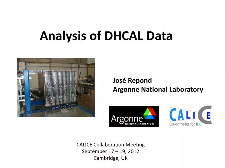
Analysis of DHCAL Data. José Repond Argonne National Laboratory. CALICE Collaboration Meeting September 17 – 19, 2012 Cambridge, UK. DHCAL Data Summary. 1 Contains a significant fraction of ‘calibration events’ 2 Contains no ‘calibration events’.

E N D
Analysis of DHCAL Data José Repond Argonne National Laboratory CALICE Collaboration Meeting September 17 – 19, 2012 Cambridge, UK
DHCAL Data Summary 1Contains a significant fraction of ‘calibration events’ 2Contains no ‘calibration events’ Data taking about x4 more efficient at CERN due to - Longer days (24 versus 12 hours) - Higher spill frequency (every 45 versus every 60 seconds) - Longer spills (9.7 versus 3.9 seconds) - More uniform extractions (no detectable microstructure) - Machine downtime similar at CERN and FNAL
Noise studies General comments - Noise rates at the level of < 1 hits per event - Response and resolution not affected by noise - Possible effect on shower shapes Hits at ground connectors
Events with hits in ground connector region Some layers have no problems Some layers are particularly bad → Reasons not entirely understood → Probably related to degraded contact between ground strip and resistive paint Exclude x=0,1 and y=20-24, 52-56, 84-88 in all analyses
Box events These events are rare, but seem to happen more often at high energies Developed two algorithms to identify and eliminate events containing boxes Burak: global analysis of all data José: developed algorithm using runs with highest rate of box events → Useful for systematic studies Conclusions from two approaches quite similar
Global analysis: Board occupancy versus Nhits 2 3 Data Data 1 4 MC MC: DHCAL Oct10 setup, assume all hits in 1ΔTS e+: 2, 4, 6, 8, 10, 12, 16, 20, 25, 32 GeV pi+: 2, 4, 6, 8, 10, 12, 16, 20, 25, 32, 40, 50, 60 GeV Cut if board occupancy>120
Global analysis → Further cuts depending on Number of hits on edge of boards Number of hits in ASICs Number of hits on edge of ASIC Analysis of 54,855,165 events (from FNAL and CERN) 608,909 rejected corresponding to 1.1% Layers identified to have a box Analysis of run 660505 (300 GeV) Use Number of hits on front-end board Number of hits on edge of front-end board Number of hits on neighboring rows of edges to identify boxes Red hits inside border Green hits on border of boards
Analysis of run 660505 →Applied to other runs Below 100 GeV Very low fraction of boxes Above 100 GeV Fraction increases dramatically Scattering of box rates probably due to varying beam intensities Reason for boxes Not yet understood Most likely related to grounding scheme Line to guide the eye Applied to simulated 100 GeV pions 23 boxes found in 10,000 events Assuming simulation close to reality → no bias introduced through box rejection
Effect of eliminating boxes on spectrum at 300 GeV After Before Lost 45% of the events Tail at high end disappeared Width reduced by 22%
Simulation of RPC response Use clean muon events Tune to average response per layer Two approaches (both useful for systematic studies) RPC_sim_3 RPC_sim_4 Spread of charge in pad plane using 2 exponentials Spread of charge in pad plane using 1 exponential 6 parameters to be tuned 4 parameters to be tuned Reproduces tail towards higher pad multiplicities Better reproduction of low multiplicity peak Does not reproduce tail towards higher multiplicities
Simulation of Positrons GEANT4 Physics list: QGSP _Bert Within MOKKA framework Fine tuning of the dcut parameter dcut: Only 1 point (to be simulated) within a radius of dcut Muon simulation not sensitive to dcut Use 4/8/10 GeV positrons to determine best dcut value
Study effect of changing gas density Note Both longitudinal and lateral shapes not well reproduced Is under investigation
Gas density affects 1) Cross section of interaction of photons in gas → to be simulated with GEANT4 → no effect on muons 2) Gain of RPC → to be simulated by RPC_sim Gas density in GEANT4 Changed corresponding to changes of ±370 C → Minimal effect on mean of hit distribution Effect of position of air gap in cassette Moved air gap from back to front of layer → Minimal effect on mean of hit distribution
Event selection General cut: 1 cluster in layer 0 with less than 12 hits BC … Longitudinal barycenter R … Average number of hits per active layer IL … Interaction layer N0 … Hits in layer 0
Spectra at -2 GeV/c Clean electrons Clean through-going muons Two peaks in pion spectrum → What are they?
Simulation of -2 GeV/c pions and muons Simulated pion/muon response fit with variable-width Gaussian Data fit to sum of pion and muon response leaving only their normalizations free Muon response depends on assumed distribution of angle of incidence Simulated pion response depends on physics list π μ
Comparison with Steel at High Energy Better resolution with Steel 37% less hits in Tungsten Note: tail towards low number of hits in Tungsten
Comparison with Simulation – RPC_sim_3 Peak positions Data = 712.9 MC = 805.5 (data not calibrated yet) Rescaling for comparison NMC x 0.885 Tail observed in data also seen in simulation
Response from 1 – 300 GeV Fits to αEβ Data not-calibrated yet
And what does Wigman’s do…. Hadron and jet detection with a dual-readout calorimeter. N. Akchurin, K. Carrell, J. Hauptman, H. Kim, H.P. Paar, A. Penzo, R. Thomas, R. Wigmans (Texas Tech. & Iowa State U. & UC, San Diego & INFN, Trieste). Feb 2005 25 pp. Nucl.Instrum.Meth. A537 (2005) 537-561 DOI: 10.1016/j.nima.2004.07.285 Quote: ‘…constant term to be added linearly to the stochastic term.’ e.g. at E=100 GeV, assuming no constant term,σ= 70%/√E , σ= 110%/√E, σ = 175%/√E
DHCAL Resolutions à la Wigmans Compare to fit to quadratic sum giving
Conclusions We have a wonderful data set with 53 Million events spanning 1 – 300 GeV in energy Detailed systematic studies of the data have begun (there is a lot to do and understand) Simulations start to look like the data The data from CERN look good Wigmans is a cheat…
Calibration of layers Assign a weight wi to each layer i Minimize resolution with wi as parameters Where n….total number of events and Method pioneered by ATLAS ← Analytical expression to calculate weights
Weight Parameters as a Function of Beam Energy Fit value provides parameter values used in weights function at each energy
Layer Weights Weights as a function of shower-layer for 10 GeV/cpions Fit to Layer number – Layer number of first interaction Currently errors on wiare calculated via a Monte Carlo smearing technique, since uncertainties in μiand Cijare correlated These errors are still under study and not quite understood yet