Download
1 / 81
830 likes | 975 Views
Using Statistics To Make Inferences 10. Summary To fit a straight line through data. Goals Given raw data, or the appropriate sums, to fit a straight line through the data. Practical Recall last weeks practical. Perform scatter plots, evaluate correlations and add regression lines. 1.

E N D
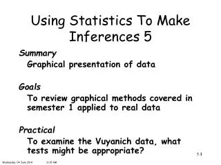
Using Statistics To Make Inferences 10 Summary To fit a straight line through data. Goals Given raw data, or the appropriate sums, to fit a straight line through the data. Practical Recall last weeks practical. Perform scatter plots, evaluate correlations and add regression lines. 1 Thursday, 13 November 201411:30 AM
Regression We wish to fit the straight line y = ax + b through our data {xi,yi: i=1,…,n} by estimating a and b. Recall these terms from lecture 9 on correlation. Note the ^ symbol denoting an estimate and the ¯ for average. 2
Example Is the height of sons related to that of their fathers? Father 63 68 70 64 66 72 67 71 68 62 Son 65 66 72 66 69 74 69 73 65 66 Which is the independent (x) variable? 3
Example Is the height of sons related to that of their fathers? Father (x) 63 68 70 64 66 72 67 71 68 62 Son (y) 65 66 72 66 69 74 69 73 65 66 Note choice of x and y variables. First plot the data. 4
Scatterplot Father (x) 63 68 70 64 66 72 67 71 68 62 Son (y) 65 66 72 66 69 74 69 73 65 66 Note that the origin is selected at a sensible value (62,65) not (0,0). 5
Calculation Father (x) 63 68 70 64 66 72 67 71 68 62 Son (y) 65 66 72 66 69 74 69 73 65 66 n = 10 Σxi = 63 + 68 + … + 62 = 671 Σyi = 65 + 66 + … + 66 = 685 Σxi2 = 632 + 682 + … + 622 = 45127 Σxiyi = 63 × 65 + 68 × 66 + … + 62 × 66 = 46047 6
Calculation Sxx n = 10 Σxi = 671 Σyi = 685 Σxi2 = 45127 Σxiyi = 46047 7
Calculation Sxy n = 10 Σxi = 671 Σyi = 685 Σxi2 = 45127 Σxiyi = 46047 8
Calculation Gradient a n = 10 Σxi = 671 Σyi = 685 Sxx = 102.9 Sxy = 83.5 Gradient or slope 9
Calculation Intercept b n = 10 Σxi = 671 Σyi = 685 Sxx = 102.9 Sxy = 83.5 Gradient or slope Intercept or constant Son = 14.05 + 0.81 ×Father 10
Results Son = 14.05 + 0.8115 × Father To produce the line select two extreme values for the x variable. Father = 72 then Son = 14.05 + 0.8115 × 72 = 72.478 Father = 62 then Son = 14.05 + 0.8115 × 62 = 64.363 11
Results Father = 72 Son = 72.48 and Father = 62 Son = 64.36 12
SPSS Analyze > Regression > Linear 13
SPSS Same intercept and gradient 14
Aside A test of extraversion was administered to two groups of subjects - 8 adolescent boys and 5 adolescent girls. Assume both populations are normally distributed. Do the two group means differ significantly at a level of 0.05? Observed data for boys 119.81 127.59 126.61 139.07 152.12 140.11 155.77 111.71 Observed data for girls 111.55 108.60 118.92 122.41 114.82 What are the key words in the question? 15
Aside C C C C C C C C C C C c A test of extraversion was administered to two groups of subjects - 8 adolescent boys and 5 adolescent girls. Assume both populations are normally distributed. Do the two group means differ significantly at a level of 0.05? Observed data for boys 119.81 127.59 126.61 139.07 152.12 140.11 155.77 111.71 Observed data for girls 111.55 108.60 118.92 122.41 114.82 16
Aside What key words describe this data? 17
Aside two sample comparison of means Which tests might be appropriate? 18
Aside C C C C C C C c z or t Which is appropriate here? Since σ is not available we use a two sample t test. 19
Example On January 28, 1986, the space shuttle Challenger was launched at a temperature of 31°F. The ensuing catastrophe was caused by a combustion gas leak through a joint in one of the booster rockets, which was sealed by a device called an O-ring. The data in the print version of the notes relate launch temperature to the number of O-rings under thermal distress for 24 previous launches. 20
Challenger's Rollout From Orbiter Processing Facility To The Vehicle Assembly Building 21
The Crew Of The Final, Ill-fated Flight Of The Challenger 22
The Challenger Breaks Apart 73 Seconds Into Its Final Mission 23
Example On January 28, 1986, the space shuttle Challenger was launched at a temperature of 31°F. The ensuing catastrophe was caused by a combustion gas leak through a joint in one of the booster rockets, which was sealed by a device called an O-ring. The data in the print version of the notes relate launch temperature to the number of O-rings under thermal distress for 24 previous launches. First plot the data. Variables, number of rings that fail and temperature Which is independent? 25
Scatterplot 26
Calculation Sxx Here the independent variable is Temp (x) and the dependent variable is Ring (y) n = 24 ΣTempi = 1680ΣRingi = 10 ΣTempi2 = 118800ΣTempi Ringi = 627 27
Calculation Sxy Here the independent variable is Temp (x) and the dependent variable is Ring (y) n = 24ΣTempi = 1680 ΣRingi = 10 ΣTempi2 = 118800 ΣTempi Ringi = 627 28
Calculation Gradient a n = 24 ΣTempi = 1680 ΣRingi = 10 Sxx = 1200 Sxy = -73 29
Calculation Intercept b n = 24 ΣTempi = 1680 ΣRingi = 10 30
Results Prediction at temp = 31 then ring = 2.789, that is at 31°F, 2.789 rings might be expected to fail! The temperature of interest is a gross extrapolation!! 31
Conclusion Richard Phillips Feynman (May 11, 1918 – February 15, 1988) was an American physicist known for his work in the path integral formulation of quantum mechanics, the theory of quantum electrodynamics, and the physics of the superfluidity of supercooled liquid helium, as well as in particle physics. For his contributions to the development of quantum electrodynamics, Feynman, jointly with Julian Schwinger and Sin-Itiro Tomonaga, received the Nobel Prize in Physics in 1965. 10.32 32
Conclusion Feynman played an important role on the Presidential Rogers Commission, which investigated the Challenger disaster. During a televised hearing, Feynman demonstrated that the material used in the shuttle's O-rings became less resilient in cold weather by immersing a sample of the material in ice-cold water. The Commission ultimately determined that the disaster was caused by the primary O-ring not properly sealing due to extremely cold weather at Cape Canaveral. 10.33 33
SPSS Same intercept and gradient 34
SPSS Scatter plots/Regression Graphs > Legacy Dialogs > Scatter/Dot Simple scatter 35
SPSS 36
SPSS To fit a line 1. Open the output file 2. Double click on the graph (the chart editor will open) 3. Click on the reference line icon 4. Click apply and close 37
What Is Multiple Regression? An example of performing a multiple regression in SPSS is presented. Multiple regression is a statistical technique that allows the prediction of a score on one variable on the basis of the scores on several other variables. 10.38 38
How Does Multiple Regression Relate To Correlation? In a previous section you met correlation and the regression line. If two variables are correlated, then knowing the score on one variable will allow you to predict the score on the other variable. The stronger the correlation, the closer the scores will fall to the regression line and therefore the more accurate the prediction. 10.39 39
How Does Multiple Regression Relate To Correlation? Multiple regression is simply an extension of this principle, where one variable is predicted on the basis of several other variables. Having more than one independent variable is useful when predicting human behaviour, as actions, thoughts and emotions are all likely to be influenced by some combination of several factors. Using multiple regression theories (or models) can be tested about precisely which set of variables is influencing behaviour. 10.40 40
When Should I Use Multiple Regression? 1. You can use this statistical technique when exploring linear relationships between dependent and independent variables – that is, when the relationship follows a straight line. 10.41 41
When Should I Use Multiple Regression? 2. The dependent variable that you are seeking to predict should be measured on a continuous scale (such as interval or ratio scale). There is a separate regression method called logistic regression that can be used for dichotomous dependent variables. 10.42 42
When Should I Use Multiple Regression? 3. The independent variables that you select should be measured on a ratio, interval, or ordinal scale. A nominal independent variable is legitimate but only if it is dichotomous, i.e. there are no more that two categories. 10.43 43
When Should I Use Multiple Regression? For example, sex is acceptable (where male is coded as 1 and female as 0) but gender identity (masculine, feminine and androgynous) could not be coded as a single variable. Instead, you would create three different variables each with two categories (masculine/not masculine; feminine/not feminine and androgynous/not androgynous). The term dummy variable is used to describe this type of dichotomous variable. 10.44 44
When Should I Use Multiple Regression? 4. Multiple regression requires a large number of observations. The number of cases (participants) must substantially exceed the number of independent variables you are using in your regression. The absolute minimum is that you have five times as many participants as independent variables. A more acceptable ratio is 10:1, but some people argue that this should be as high as 40:1 for some statistical selection methods. 10.45 45
Terminology There are certain terms that need to clarifying to allow you to understand the results of this statistical technique. 10.46 46
Beta (standardised regression coefficients) The beta value is a measure of how strongly each independent variable influences the dependent variable. The beta is measured in units of standard deviation. For example, a beta value of 2.5 indicates that a change of one standard deviation in the independent variable will result in a change of 2.5 standard deviations in the dependent variable. Thus, the higher the beta value the greater the impact of the independent variable on the dependent variable. 10.47 47
Beta (standardised regression coefficients) When you have only one independent variable in your model, then beta is equivalent to the correlation coefficient between the independent and the dependent variable. When you have more than one independent variable, you cannot compare the contribution of each independent variable by simply comparing the correlation coefficients. The beta regression coefficient is computed to allow you to make such comparisons and to assess the strength of the relationship between each independent variable to the dependent variable. 10.48 48
R, R Square, Adjusted R Square R is a measure of the correlation between the observed value and the predicted value of the dependent variable. R Square (R2) is the square of this measure of correlation and indicates the proportion of the variance in the dependent variable which is accounted for by the model. In essence, this is a measure of how good a prediction of the dependent variable can be made by knowing the independent variables. 10.49 49
R, R Square, Adjusted R Square However, R square tends to somewhat over-estimate the success of the model when applied to the real world, so an Adjusted R Square value is calculated which takes into account the number of variables in the model and the number of observations (participants) the model is based on. This Adjusted R Square value gives the most useful measure of the success of the model. If, for example an Adjusted R Square value of 0.75 it can be said that the model has accounted for 75% of the variance in the dependent variable. 10.50 50