Download
1 / 14
140 likes | 298 Views
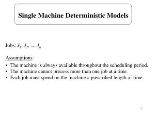
Single Machine Deterministic Models. Jobs: J 1 , J 2 , ..., J n Assumptions : The machine is always available throughout the scheduling period. The machine cannot process more than one job at a time. Each job must spend on the machine a prescribed length of time. S ( t ). 3. 2. 1.

E N D
Single Machine Deterministic Models • Jobs: J1, J2, ..., Jn • Assumptions: • The machine is always available throughout the scheduling period. • The machine cannot process more than one job at a time. • Each job must spend on the machine a prescribed length of time.
S(t) 3 2 1 t J2 J3 J1 ...
Requirements that may restrict the feasibility of schedules: • precedence constraints • no preemptions • release dates • deadlines • Whether some feasible schedule exist? NP hard Objective function f is used to compare schedules. f(S) < f(S') whenever schedule S is considered to be better than S' problem of minimising f(S) over the set of feasible schedules.
1. Completion Time Models Due date related objectives: 2. Lateness Models 3. Tardiness Models 4. Sequence-Dependent Setup Problems
Completion Time Models Contents 1. An algorithm which gives an optimal schedule with the minimum total weighted completion time 1 || wjCj 2. An algorithm which gives an optimal schedule with the minimum total weighted completion time when the jobs are subject to precedence relationship that take the form of chains 1 | chain | wjCj
Literature: • Scheduling, Theory, Algorithms, and Systems, Michael Pinedo, Prentice Hall, 1995, or new: Second Addition, 2002, Chapter 3.
1 || wjCj Theorem.The weighted shortest processing time first rule (WSPT) isoptimal for 1 || wjCj WSPT: jobs are ordered in decreasing order of wj/pj The next follows trivially: The problem 1 || Cj is solved by a sequence S with jobs arranged innondecreasing order of processing times.
which implies that wj pk < wk pj Proof. By contradiction. S is a schedule, not WSPT, that is optimal. j and k are two adjacent jobs such that S: ... ... k j t + pj + pk t ... ... S’ k j t + pj + pk t S: (t+pj) wj + (t+pj+pk) wk = t wj + pj wj + t wk + pj wk + pk wk S’: (t+pk) wk + (t+pk+pj) wj = t wk + pk wk + t wj + pk wj + pj wj the completion time for S’ < completion time for Scontradiction!
1 | chain | wjCj chain 1: 1 2 ... k chain 2: k+1 k+2 ... n Lemma. If the chain of jobs 1,...,k precedes the chain of jobs k+1,...,n. Let l* satisfy factor of chain 1,...,k l* is the job that determines the factor of the chain
Lemma. If job l* determines (1,...,k) , then there exists an optimalsequence that processes jobs 1,...,l* one after another withoutinterruption by jobs from other chains. Algorithm Whenever the machine is free, select among the remaining chainsthe one with the highest factor. Process this chain up to and includingthe job l* that determines its factor.
Example chain 1: 1 2 3 4 chain 2: 5 6 7 factor of chain 1 is determined by job 2: (6+18)/(3+6)=2.67 factor of chain 2 is determined by job 6: (8+17)/(4+8)=2.08 chain 1 is selected: jobs 1, 2 factor of the remaining part of chain 1 is determined by job 3:12/6=2 factor of chain 2 is determined by job 6: 2.08 chain 2 is selected: jobs 5, 6
factor of the remaining part of chain 1 is determined by job 3: 2 factor of the remaining part of chain 2 is determined by job 7:18/10=1.8 chain 1 is selected: job 3 factor of the remaining part of chain 1 is determined by job 4: 8/5=1.6 factor of the remaining part of chain 2 is determined by job 7: 1.8 chain 2 is selected: job 7 job 4 is scheduled last the final schedule: 1, 2, 5, 6, 3, 7, 4
1 | prec | wjCj • Polynomial time algorithms for the more complex precedence constraints than the simple chains are developed. • The problems with arbitrary precedence relation are NP hard. • 1 | rj, prmp | wjCj preemptive version of the WSPT rule does not always lead to an optimal solution, the problem is NP hard • 1 | rj, prmp | Cj preemptive version of the SPT rule is optimal • 1 | rj | Cj is NP hard
Summary • 1 || wjCj WSPT rule • 1 | chain | wjCj a polynomial time algorithm is given • 1 | prec | wjCj with arbitrary precedence relation is NP hard • 1 | rj, prmp | wjCj the problem is NP hard • 1 | rj, prmp | Cj preemptive version of the SPT rule is optimal • 1 | rj | Cj is NP hard