Download
1 / 26
260 likes | 264 Views
Lower resolution X-ray spectroscopy. Keith Arnaud NASA/GSFC & UMCP. Practical X-ray spectroscopy. Most X-ray spectra are of moderate or low resolution (eg Chandra ACIS or XMM-Newton EPIC). However, the spectra generally cover a bandpass of more than 1.5 decades in energy.

E N D
Lower resolution X-ray spectroscopy Keith Arnaud NASA/GSFC & UMCP X-ray Astronomy School 2002
Practical X-ray spectroscopy Most X-ray spectra are of moderate or low resolution (eg Chandra ACIS or XMM-Newton EPIC). However, the spectra generally cover a bandpass of more than 1.5 decades in energy. Moreover, the continuum shape often provides important physical information. Therefore, unlike in the optical, most uses of X-ray spectra have involved a simultaneous analysis of the entire spectrum rather than an attempt to measure individual line strengths. X-ray Astronomy School 2002
Martin Elvis Proportional counter e.g. ROSAT PSPC 3C 273 Optical Spectrum CCD e.g. Chandra ACIS Grating X-ray Astronomy School 2002
Can we start with these… and deduce this ? X-ray Astronomy School 2002
Can we start with this… X-ray Astronomy School 2002
and deduce this X-ray Astronomy School 2002
The Basic Problem Suppose we observe D(I) counts in channel I (of N) from some source. Then : D(I) = T ∫ R(I,E) A(E) S(E) dE • T is the observation length (in seconds) • R(I,E) is the probability of an incoming photon of energy E being registered in channel I (dimensionless) • A(E) is the energy-dependent effective area of the telescope and detector system (in cm2) • S(E) is the source flux at the front of the telescope (in photons/cm2/s/keV X-ray Astronomy School 2002
An example R(I,E) photopeak photopeak fluorescence fluourescence escape escape X-ray Astronomy School 2002
The Basic Problem II D(I) = T ∫ R(I,E) A(E) S(E) dE We assume that T, A(E) and R(I,E) are known and want to solve this integral equation for S(E). We can divide the energy range of interest into M bins and turn this into a matrix equation : Di= T ∑Rij Aj Sj where Sj is now the flux in photons/cm2/s in energy bin J. We want to find Sj. X-ray Astronomy School 2002
The Basic Problem III Di = T ∑Rij Aj Sj The obvious tempting solution is to calculate the inverse of Rij, premultiply both sides and rearrange : (1/T Aj) ∑(Rij)-1Di = Sj This does not work ! The Sj derived in this way are very sensitive to slight changes in the data Di. This is a great method for amplifying noise. X-ray Astronomy School 2002
A (brief) Mathematical Digression This should not have come as a surprise to anyone with any data analysis experience. This is known as the “remote sensing problem” and arises in many areas of astronomy as well as eg geophysics and medical imaging. In mathematics the integral is known as a Fredholm equation of the first kind. Tikhonov showed that such equations can be solved using “regularization” - applying a priori knowledge to damp the noise. A familiar example is maximum entropy but there are a host of others. Some of these have been tried on X-ray spectra - none have had any impact on the field. X-ray Astronomy School 2002
Forward-fitting • The standard method of analyzing X-ray spectra is “forward-fitting”. This comprises the following steps… • Calculate a model spectrum. • Multiply the result by an instrumental response matrix. • Compare the result with the actual observed data by calculating some statistic. • Modify the model spectrum and repeat till the best value of the statistic is obtained. X-ray Astronomy School 2002
Define Model Forward-fitting algorithm Calculate Model Convolve with detector response Change model parameters Compare to data X-ray Astronomy School 2002
This only works if the model spectrum can be expressed in a reasonably small number of parameters so that the model can be varied in some sensible fashion. The aim of the forward-fitting is then to obtain the best-fit and confidence ranges of these parameters (cf Peter’s talks). X-ray Astronomy School 2002
Spectral fitting programs • XSPEC- part of HEAsoft. General spectral fitting program with many models available. • Sherpa - part of CIAO. Multi-dimensional fitting program which includes the XSPEC model library and can be used for spectral fitting. • SPEX - from SRON in the Netherlands. Spectral fitting program specialising in collisional plasmas and high resolution spectroscopy. • ISIS - from the MIT Chandra HETG group. Mainly intended for the analysis of grating data. X-ray Astronomy School 2002
Models All models are wrong, but some are useful - George Box X-ray spectroscopic models are usually built up from individual components. These can be thought of as two basic types -additive (an emission component e.g. blackbody, line,…) or multiplicative (something which modifies the spectrum e.g. absorption). Model = M1 * M2 * (A1 + A2 + M3*A3) + A4 X-ray Astronomy School 2002
Additive Models • Basic additive (emission) models include : • blackbody • thermal bremsstrahlung • power-law • collisional plasma • Gaussian or Lorentzian lines • There are many more models available covering specialised topics such as accretion disks, comptonized plasmas, non-equilibrium ionization plasmas, multi-temperature collisional plasmas… X-ray Astronomy School 2002
Multiplicative (and Other) Models • and multiplicative models include : • photoelectric absorption due to our Galaxy • photoelectric absorption due to ionized material • high energy exponential roll-off. • edge with 1/E3 roll-off. • XSPEC also has a couple of other types of model components (convolution, mixing) which are used like a multiplicative model but perform more complicated operations on the current model. X-ray Astronomy School 2002
Roll Your Own Models There is a simple XSPEC model interface which enables astronomers to write new models and fit them to their data. You can write your own subroutine and hook it in - the subroutine takes in the energies on which to calculate the model and writes out the fluxes (in photons/cm2/s). In addition, there is also a standard format for files containing model spectra so these too can be fit to data without having to add new routines to XSPEC. X-ray Astronomy School 2002
Finding the best-fit Finding the best-fit means minimizing the statistic value. There are many algorithms available to do this in a computationally efficient fashion (see Numerical Recipes). Most methods used to find the best-fit are local i.e. they use some information around the current parameters to guess a new set of parameters. All these methods are liable to get stuck in a local minimum. Watch out for this ! The more complicated your model and the more highly correlated the parameters then the more likely that the algorithm will not find the absolute best-fit. X-ray Astronomy School 2002
Finding the best-fit II Sometimes you can spot that you are stuck in a local minimum by using the XSPEC error or steppar commands. These both step through parameter values, error in the vicinity of the current best-fit and steppar over a user-defined grid, and thus can stumble across a better fit. Crude but sometimes effective. You can do this in a semi-automated fashion by using a local minimization algorithm and following this with the error command with the ability to restart if a new minimum is found during the search. X-ray Astronomy School 2002
Global Minimization There are global minimization methods available - simulated annealing, genetic algorithms, … - but they require many function evaluations (so are slow) and are still not guaranteed to find the true minimum. A new technique called Markov Chain Monte Carlo, which provides an intelligent sampling of parameter space, looks promising but it is not yet widely available (i.e. I’ve not added it to XSPEC - yet). X-ray Astronomy School 2002
Markov Chain Monte Carlo A Markov Chain is a sequence of random variables {X0, X1, X2, …} such that each state Xt+1 is sampled from a distribution p(Xt+1|Xt) which depends only on the current state Xt. The fundamental theorem of Markov Chains shows that for large enough t the Xt are drawn from a stationary distribution which is independent of t and the starting point of the chain. The MCMC method then consists of setting up a Markov Chain such that the stationary distribution is the distribution of interest. The Markov Chain values then provide a sampling of the distribution which we can use for integration or characterization. X-ray Astronomy School 2002
Markov Chain Monte Carlo II Constructing such Markov Chains turns out to be remarkably simple. The method was first developed in 1953 by Metropolis et al. (in the context of statistical physics) and generalized in 1970 by Hastings. • Suppose that our target distribution is p(X). We are at Xt in the chain. • Sample a candidate point Y from a proposal distribution q(Xt). • Accept Y with a probability p(Y)q(X|Y)/p(X)/q(Y|X). • If the candidate is accepted set Xt+1=Y otherwise Xt+1=Xt. X-ray Astronomy School 2002
Markov Chain Monte Carlo III Remarkably, q can be any distribution and the stationary distribution of the chain will still be p. However, it should be chosen so that the chain converges quickly (a short “burn-in”) and mixes well ie it samples all parts of the distribution p. There are a number of canonical choices for q and this is an active area of research in the statistical community. X-ray Astronomy School 2002
Final Advice and Admonitions • Remember that the purpose of spectral fitting is to attain understanding, not fill up tables of numbers. • Don’t bin up your data - especially in a way that is dependent on the data values (eg group min 15). • Don’t misuse the F-test. • Try to test whether you really have found the best-fit. X-ray Astronomy School 2002