Download

1 / 63
630 likes | 725 Views
PID-tuning using the SIMC rules. Sigurd Skogestad Department of Chemical Engineering, NTNU, Trondheim, Norway. Salamanca, Spain, Feb. 2017. TexPoint fonts used in EMF. Read the TexPoint manual before you delete this box.: A A A A A A A A A. Arctic circle. North Sea. Trondheim. SWEDEN.

E N D
PID-tuning using the SIMC rules Sigurd Skogestad Department of Chemical Engineering, NTNU, Trondheim, Norway Salamanca, Spain, Feb. 2017 TexPoint fonts used in EMF. Read the TexPoint manual before you delete this box.: AAAAAAAAA
Arctic circle North Sea Trondheim SWEDEN NORWAY Oslo DENMARK GERMANY UK
Operation hierarchy RTO CV1 MPC CV2 PID u (valves)
Outline • First-order plus delay model. • PID-control. • SIMC PI(D)-rule • Optimal PI controller • Comparison of SIMC with optimal PI • Improved SIMC-PI for time-delay process • Non-PID control of first-order plus delay process: Better with IMC / Smith Predictor / MPC? (no) • Example: Level control • Conclusion
First-order + delay model for PI-control Second-order model for PID-control Recommend: Use second-order model only if ¿2>µ 1. Need a model for tuning
MODEL, Approach 1 Step response experiment • Make step change in one u (MV) at a time • Record the output (s) y (CV) y u MV = manipulated variable (input) CV = controlled variable (output)
RESULTING OUTPUT y (CV) k’=k/1 STEP IN INPUT u (MV) Identify k, 1 and from step response If doesn’t settle: Don’t need k and 1.Stop experiment at about 8 x and assume integrating process : Delay - Time where output does not change 1: Time constant - Additional time to reach 63% of final change k : steady-state gain = y(1)/ u k’ : slope after response “takes off” = k/1
MODEL, Approach 2 Closed-loop setpoint response with P-controller with about 20-40% overshoot Kc0=1.5 Δys=1 Δy∞ • OBTAIN DATA IN RED (first overshoot • and undershoot), and then: • tp=4.4, dyp=0.79; dyu=0.54, Kc0=1.5, dys=1 • dyinf = 0.45*(dyp + dyu) • Mo =(dyp -dyinf)/dyinf % Mo=overshoot (about 0.3) • b=dyinf/dys • A = 1.152*Mo^2 - 1.607*Mo + 1.0 • r = 2*A*abs(b/(1-b)) • %2. OBTAIN FIRST-ORDER MODEL: • k = (1/Kc0) * abs(b/(1-b)) = 0.99 • theta = tp*[0.309 + 0.209*exp(-0.61*r)] = 1.68 • tau = theta*r = 3.03 Δyp=0.79 Δyu=0.54 tp=4.4 Similar to Ziegler-Nichols experiment but get more information Ref: Shamssuzzoha and Skogestad (JPC, 2010) + modification by C. Grimholt (PID-book 2012)
Start with complicated stable model on the form Want to get a simplified model on the form Most important parameter is the “effective” delay MODEL, Approach 3 Model reduction of more complicated model
MODEL, Approach 3 Example 1 Half rule
MODEL, Approach 3 original 1st-order+delay
MODEL, Approach 3 2 half rule
MODEL, Approach 3. HALF RULE original 1st-order+delay 2nd-order+delay
Time domain (“ideal” PID) Laplace domain (“ideal”/”parallel” form) For our purposes. Simpler with cascade form Usually τD=0. Then the two forms are identical. Only two parameters left (Kc and τI) How difficult can it be to tune??? Surprisingly difficult without systematic approach! 2. PID controller e
Trans. ASME, 64, 759-768 (Nov. 1942). Comment: Similar to SIMC for integrating process with ¿c=0: Kc = 1/k’ 1/µ ¿I = 4 µ Disadvantages Ziegler-Nichols: • Aggressive settings • No tuning parameter • Poor for processes with large time delay (µ)
Disadvantage IMC-PID: • Many rules • Poor disturbance response for «slow» processes (with large ¿1/µ)
Motivation for developing SIMC PID tuning rules • The tuning rules should be well motivated, and preferably be model-based and analytically derived. • They should be simple and easy to memorize. • They should work well on a wide range of processes.
3. SIMC PI tuning rule • Approximate process as first-order with delay (e.g., use “half rule”) • k = process gain • ¿1 = process time constant • µ = process delay • Derive SIMC tuning rule*: Open-loop step response c¸ -: Desired closed-loop response time (tuning parameter) Integral time rule combines well-known rules: IMC (Lamda-tuning): Same as SIMC for small ¿1 (¿I = ¿1) Ziegler-Nichols: Similar to SIMC for large ¿1 (if we choose ¿c= 0; aggressive!) Reference: S. Skogestad, “Simple analytic rules for model reduction and PID controller design”, J.Proc.Control, Vol. 13, 291-309, 2003 (*) “Probably the best simple PID tuning rules in the world”
Derivation SIMC tuning rule. Basis: Direct synthesis (IMC) for setpoints Closed-loop response to setpoint change: Idea: Specify desired response: and from this get the controller. ……. Algebra:
NOTE: Setting T(0)=1 (steady-state gain = 1) gives integral action.
d u y c g Integral time • Found: Integral time = dominant time constant (I = 1) (IMC-rule) • Works well for setpoint changes • Needs to be modified (reduced) for integrating disturbances Example. “Almost-integrating process” with disturbance at input: G(s) = e-s/(30s+1) Original integral time I = 30 gives poor disturbance response Try reducing it!
IMC-rule: I = 1=30 Effect of integral time on closed-loop response Setpoint change (ys=1) at t=0 Input disturbance (d=1) at t=20
SIMC: Integral time correction • Setpoints: ¿I=¿1(“IMC-rule”). Want smaller integral time for disturbance rejection for “slow” processes (with large ¿1), but to avoid “slow oscillations” must require: • Derivation: • Conclusion SIMC:
Conclusion: SIMC-PID Tuning Rules One tuning parameter: c • Note: • Recommend derivative action (PID) only for «dominant» second-order proceses» withτ2>θ. • Otherwise, addτ2 to θ and use PI.
Selection of tuning parameter c • Tuning parameter: c = desired closed-loop response time • Choice c=(“tight control”) gives good balance between performance (IAE) and robustness • Other cases: Select c > (“smooth control”) for • slower control • smoother input usage • less disturbing effect on rest of the plant • less sensitivity to measurement noise • better robustness S. Skogestad, ``Tuning for smooth PID control with acceptable disturbance rejection'', Ind.Eng.Chem.Res, 45 (23), 7817-7822 (2006).
Example. Integrating process with delay=1. G(s) = e-s/s. Model: k’=1, =1, 1=1 SIMC-tunings with c with ==1: IMC has I=1 Ziegler-Nichols is usually a bit aggressive Setpoint change at t=0c Input disturbance at t=20
Approximate as first-order model: • k=1, 1 = 1+0.1=1.1, =0.1+0.04+0.008 = 0.148 • Get SIMC PI-tunings (c=): Kc = 1 ¢ 1.1/(2¢ 0.148) = 3.71, I=min(1.1,8¢ 0.148) = 1.1 • Approximate as second-order model: • k=1, 1 = 1, 2=0.2+0.02=0.22, =0.02+0.008 = 0.028 • Get SIMC PID-tunings (c=): Kc = 1 ¢ 1/(2¢ 0.028) = 17.9, I=min(1,8¢ 0.028) = 0.224, D=0.22
SIMC: Tuning parameter (¿c) correlates nicely with robustness measures PM Ms 60o 1.6 1 1 DM= D/ GM 2 3 1 1 c / c /
But: How good is really the SIMC rule? Want to compare with: • Optimal PI-controller for class of first-order with delay processes
4. Optimal PID controller High controller gain (“tight control”) Low controller gain (“smooth control”) • Multiobjective. Tradeoff between • Output performance • Robustness • Input usage • Noise sensitivity Our choice: • Quantification • Output performance: • Rise time, overshoot, settling time • IAE or ISE for setpoint/disturbance • Robustness: Ms, Mt, GM, PM, Delay margin, … • Input usage: ||KSGd||, TV(u) for step response • Noise sensitivity: ||KS||, etc. J = avg. IAE for setpoint/disturbance Ms = peak sensitivity
Optimal PI-controller Optimal sensitivity function, S = 1/(gc+1) Ms=2 |S| Ms=1.59 Ms=1.2 frequency
Output performance (J) IAE = Integrated absolute error = ∫|y-ys|dt, for step change in ys or d Cost J(c) is independent of: • process gain (k) • setpoint (ys or dys) and disturbance (d) magnitude • unit for time
Optimal PI-controller Optimal closed-loop response Ms=1.59 IAE Setpoint change at t=0, Input disturbance at t=20, g(s)=k e-θs/(1s+1), Time delay θ=1
Optimal PI-controller Optimal closed-loop response Ms=1.2 IAE Setpoint change at t=0, Input disturbance at t=20, g(s)=k e-θs/(1s+1), Time delay θ=1
Optimal PI-controller Optimal PI-controller: Minimize J=IAE for given Ms Chriss Grimholt and Sigurd Skogestad. "Optimal PI-Control and Verification of the SIMC Tuning Rule". Proceedings IFAc conference on Advances in PID control (PID'12), Brescia, Italy, 28-30 March 2012.
Uninteresting Pareto-optimal PI Infeasible
Optimal PI-controller Optimal performance (J) vs. Ms
Comparison of J vs. Ms for optimal and SIMC-PI for 4 processes
Optimal PI-controller Optimal PI-settings vs. process time constant (1 /θ)
Conclusion (so far): How good is really the SIMC rule? • Varying C gives (almost) Pareto-optimal tradeoff between performance (J) and robustness (Ms) • C = θ is a good ”default” choice • Not possible to do much better with any other PI-controller! • Exception: Time delay process
6. Can the SIMC-rule be improved? Yes, for time delay process
Optimal PI-controller Optimal PI-settings (small 1) 0.33 Time-delay process SIMC: I=1=0
Step response for time delay process Optimal PI θ=1 NOTE for time delay process: Setpoint response = disturbance responses = input response
Two “Improved SIMC”-rules that give optimal for pure time delay process 1. Improved PI-rule: Add θ/3 to 1 1. Improved PID-rule: Add θ/3 to 2