Download
1 / 26
270 likes | 589 Views
Academy of Economic Studies Bucharest Doctoral School of Finance and Banking. Measuring market risk: a copula and extreme value approach. Supervisor Professor Mois ă Altăr. M. Sc. Student A lexandru St ângă. July 2007. Contents. Goal Literature review Methodology

E N D
Academy of Economic Studies BucharestDoctoral School of Finance and Banking Measuring market risk: a copula and extreme value approach Supervisor Professor Moisă Altăr M. Sc. Student Alexandru Stângă July 2007
Contents • Goal • Literature review • Methodology • Estimation and results • Conclusion
Goal Measuring the risk of a portfolio composed of 5 Romanian stocks traded on the Bucharest Stock Exchange • Modelling individual return series using GARCH methods and extreme value theory and the dependence structure using the notion of copula in order to simulate a portfolio returns distribution • Accurately capturing the data generating process for each return series in order to efficiently estimate VAR and ES values • Backtesting for precision of the risk measure selected
Literature review Main sources: • McNeil, A.J. and R.Frey (2000)„Estimation of Tail-Related Risk Measures for Heteroscedastic Financial Time Series: an Extreme Value Approach” • Nyström, K. and J. Skoglund (2002a), „A Framework for Scenariobased Risk Management”
Methodology - GARCH • conditional mean equation • conditional variance equation • Leverage coefficient introduced by Glosten, Jagannathan and Runkle (1993)
Methodology – Extreme Value Theory Peak-over-threshold model For a sample of observations, rt, t = 1, 2, . . , n with a distribution function F(x) = Pr{rt ≤ x} and a high-threshold u, the exceedances over this threshold occur when rt > u for any t = 1, 2, . . , n. An excess over u is defined by y = rt − u. The theorem of Balkema and de Haan (1974) and Pickands (1975) shows that for sufficiently high threshold u, the distribution function of the excess may be approximated by the Generalized Pareto Distribution (GPD): ξ- shape parameter; σ scale parameter; υ location parameter
Methodology – Copulas • A joint distribution can be decomposed into marginal distributions and a dependence structure represented by a copula function. • Multivariate Gaussian Copula: where ΦR is the standard multivariate normal distribution with correlation matrix R; Φ-1(u) is the inverse of the normal cumulative distribution function • Multivariate Student’s t Copula where TR,v denotes the standard multivariate Student’s t distribution with correlation matrix R and v degrees of freedom; tv-1(u) denotes the inverse of the Student’s t cumulative distribution function
Methodology – Measures of risk Value-at-Risk Measures the worst loss to be expected of a portfolio over a given time horizon at a given confidence level Advantages: • simple and intuitive method of evaluating risk Disadvantages: • gives only an upper limit on the losses given a confidence level • tells nothing about the potential size of the loss if this upper limit is exceeded • not a coherent measure of risk (Artzner et al. 1997, 1998) Expected Shortfall Measures the average loss to be expected of a portfolio over a given time horizon provided that VaR has been exceeded.
Estimation and results - Data • Five Romanian equities traded on the Bucharest Stock Exchange (symbols: SIF1, SIF2, SIF3, SIF4, SIF5) • Selection criteria • high market liquidity • long time series with few missing values • high volatility periods • Period: 01.2001 – 06.2007; 1564 observations • The price series are adjusted for corporate events
Estimation and results - Overview • GARCH coefficients estimation • Construction of semi-parametric distributions for the standardized residuals (zt) • Extreme value modelling of the tails (Generalized Pareto Distributions) • Kernel smoothing of the interior • Student’s t Copula calibration • Simulation of the conditional portfolio distribution • Value-at-risk and Expected Shortfall estimation • Value-at-Risk backtesting
Estimation and results - GARCH • Testing for the autocorrelation of returns and the presence of a volatility clustering effect • Sample autocorrelation function plot (returns and squared returns)
Estimation and results - GARCH Testing for the autocorrelation of returns and the presence of a volatility clustering effect • Ljung Box test for randomness (returns and squared returns) Null Hypothesis:none of the autocorrelation coefficients up to lag 20 are different from zero
Estimation and results - GARCH Initial model
Estimation and results - GARCH Testing for the autocorrelation of the standardized residuals ( ) and the presence of a volatility clustering effect • Ljung Box test for randomness - standardized residuals ( ) and squared standardized residuals ( ) Null Hypothesis:none of the autocorrelation coefficients up to lag 20 are different from zero
Estimation and results – Extreme Value Assumptions: • a skewed standardized residual distribution • an overestimation of the tail heaviness by the Student’s t distribution
Estimation and results – Extreme Value • Peak-over-threshold method fits the tails better than the Student’s t distribution estimated by the GARCH model • Asymmetric standardized residual distribution with a heavier lower tail.
Estimation and results – Extreme Value • Construction of the semi-parametric distributions • Generalized Pareto fitted tails • Kernel Smoothed interior • Building of pseudo cumulative distribution functions (CDF) and inverse cumulative distribution functions (ICDF) for Monte Carlo simulation
Estimation and results – Copula Calibrating the parameters of the Student’s t copula with canonical maximum likelihood (CML) method. • CML method allows for an estimation of the copula parameters without an assumption about the marginal distributions • The standardized residuals X = (X1t,…, Xnt)t=1T are transformed into uniform variates using the marginal distribution functions (pseudo-CDF): ut = (ut1,….., utn) = [F1(X1t),…., Fn(Xnt)]. • The vector of copula parameters α are estimated via the following relation:
Estimation and results – Copula • DoF parameter estimated with the profile log likelihood method • Positive correlation of the series • Low degrees of freedom parameter implies a high tail dependence.
Estimation and results – Simulation Simulation of a conditional distribution for the portfolio with the semi-parametric marginal distributions and the dependence structure given by the t-copula • 3000 trials are generated from a multivariate Student’s t distribution with the same correlation matrix and degrees of freedom parameters as those estimated with the t-copula • transformation of each simulated series into the corresponding semi-parametrical distribution. • building the conditional distribution of the portfolio by reintroducing the volatility with the GARCH models
Estimation and results – Risk measures Value at Risk is estimated by taking the relevant quantile qα of the conditional portfolio distribution*: VaRα = qα Expected Shortfall is estimated by using the following formula**: * if the losses are marked with a positive sign and gains with a negative sign ** where n represents the number of trials
Estimation and results – Value-at-risk backtesting Value-at-Risk backtesting • 1 day horizon • estimation for the last 500 days of the series • fixed data sample of 1000 observations • for each day all the parameters are re-estimated
Conclusion • the GARCH models explain well the autocorrelation found in the return series and the volatility clustering effect • the distributions of the innovations are asymmetric with heavy lower tails and thin upper tails • the GPD describes the tails of the standardized residuals better than the Student’s t-distribution • the backtesting results for Value-at-Risk are not conclusive but give an indication of a possible underestimation of the risk at 95% confidence level • Further research: • estimation of risk for different risk factors • methodology improvement