Download
1 / 28
300 likes | 579 Views
PART III The Core of Macroeconomic Theory. The level of GDP, the overall price level, and the level of employment—three chief concerns of macroeconomists—are influenced by events in three broadly defined “markets”: Goods-and-services market Financial (money) market Labor market.

E N D
PART IIIThe Core of Macroeconomic Theory • The level of GDP, the overall price level, and the level of employment—three chief concerns of macroeconomists—are influenced by events in three broadly defined “markets”: • Goods-and-services market • Financial (money) market • Labor market
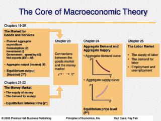
PART IIIThe Core of Macroeconomic Theory FIGURE III.1 The Core of Macroeconomic Theory We build up the macroeconomy slowly. In Chapters 8 and 9, we examine the market for goods and services. In Chapters 10 and 11, we examine the money market. Then in Chapter 12, we bring the two markets together, in so doing explaining the links between aggregate output (Y) and the interest rate (r), and derive the aggregate demand curve. In Chapter 13, we introduce the aggregate supply curve and determine the price level (P). We then explain in Chapter 14 how the labor market fits into the macroeconomic picture.
Aggregate Expenditureand Equilibrium Output CHAPTER OUTLINE The Keynesian Theory of Consumption Planned Investment (I) The Determination of Equilibrium Output (Income) The Multiplier Adapted from: Fernando & Yvonn Quijano
8.1 Aggregate Expenditure and Equilibrium Output aggregate output The total quantity of goods and services produced (or supplied) in an economy in a given period. aggregate income The total income received by all factors of production in a given period. In any given period, there is an exact equality between aggregate output (production) and aggregate income. Y = aggregate output (income)
8.2 The Keynesian Theory of Consumption FIGURE 8.1 A Consumption Function for a Household A consumption function for an individual household shows the level of consumption at each level of household income.
8.2 The Keynesian Theory of Consumption Consumption function: C = a + bY FIGURE 8.2 An Aggregate Consumption Function The upward slope indicates that higher levels of income lead to higher levels of consumption spending.
8.2 The Keynesian Theory of Consumption marginal propensity to consume (MPC) That fraction of a change in income that is consumed, or spent. aggregate saving (S) The part of aggregate income that is not consumed. S ≡Y– C marginal propensity to save (MPS) That fraction of a change in income that is saved. MPC + MPS≡ 1
8.2 The Keynesian Theory of Consumption • E.g. Suppose C = 100 + 0.75 Y • When Y0 = $800, C0 = 100 + 0.75 (800) = $700 • S0 = 800 – 700 = $100 • When aggregate income increased by $200 (Y=200) to $1000, how much of that extra $200 will be spent? How much will be saved? • When Y1= $1000, C1 = 100 + 0.75 (1000) = $850 • S1 = 1000 – 850 = $150 • Y = Y1 - Y0 = $200C = C1 - C0 = $150S = S1 - S0 = $50 • MPC = C/ Y = 150/200 = 0.75 MPS = S/ Y = 50/200 = 0.25
8.2 The Keynesian Theory of Consumption FIGURE 8.3 The Aggregate Consumption Function Derived from the Equation C = 100 + .75Y
8.2 The Keynesian Theory of Consumption FIGURE 8.4 Deriving the Saving Function from the Consumption Function in Figure 8.3 When Y = C, S = 0 When Y < C, S is negative When Y > C, S is positive
8.2 The Keynesian Theory of Consumption Other Determinants of Consumption • In practice, the decisions of households on how much to consume in a given period are also affected by: • their wealth • the interest rate • their expectations of the future (better job prospect, government future policy announcements).
8.3 Planned Investment (I) FIGURE 8.5 The Planned Investment Function For the time being, we will assume that planned investment is fixed. It does not change when income changes, so its graph is a horizontal line.
8.4 The Determination of Equilibrium Output (Income) planned aggregate expenditure (AE) The total amount the economy plans to spend in a given period. AE ≡ C + I At equilibrium, aggregate output = planned aggregate expenditure Y = AE Y = C + I
8.4 The Determination of Equilibrium Output (Income) FIGURE 8.6 Equilibrium Aggregate Output Y < C + I Y > C + I
8.4 The Determination of Equilibrium Output (Income) Adjustment to Equilibrium aggregate output > planned aggregate expenditure Y > C + I If output is greater than planned spending, there will be unplanned increases in inventories. In this case, firms will respond by reducing output. As output falls, income falls, consumption falls, and so on, until equilibrium is restored, with Y lower than before.
8.4 The Determination of Equilibrium Output (Income) Adjustment to Equilibrium aggregate output < planned aggregate expenditure Y < C + I If output is less than planned aggregate expenditure, unplanned inventory reductions have occurred. In this case, firms will respond by increasing output. As output increases, income rises, consumption rises, and so on, until equilibrium is restored, with Y higher than before
8.4 The Determination of Equilibrium Output (Income) Adjustment to Equilibrium Suppose C = 100 + 0.75Y, and I = 25 At equilibrium, Y = C + I = (100 + 0.75Y) + 25 = 125 + 0.75Y 0.25Y = 125 Y = 125 / 0.25 = 500 The equilibrium level of output is 500
8.4 The Determination of Equilibrium Output (Income) The Saving/Investment Approach to Equilibrium Given that: Y ≡ C + S At equilibrium, Y = C + I C + S = C + I S = I only when planned investment equals saving will there be equilibrium.
8.4 The Determination of Equilibrium Output (Income) Adjustment to Equilibrium Suppose C = 100 + 0.75Y, and I = 25 Given that Y ≡ C + S = (100 + 0.75Y) + S S = -100 + 0.25Y At equilibrium, S = I -100 + 0.25Y = 25 0.25Y = 125 Y = 125 / 0.25 = 500 The equilibrium level of output is 500
8.4 The Determination of Equilibrium Output (Income) The Saving/Investment Approach to Equilibrium FIGURE 8.7 The S = I Approach to Equilibrium Saving and planned investment are equal at Y = 500.
8.5 The Multiplier multiplier The ratio of the change in the equilibrium level of output to a change in some exogenous variable. E.g. Investment multiplier = Y/ I Government spending multiplier = Y/ G Tax multiplier = Y/ T exogenous variable A variable that is assumed not to depend on the state of the economy—that is, it does not change when the economy changes. For simplicity, let us consider planned investment (I) is exogenous. Suppose I increases by 25 to 50, how much will the equilibrium level of output (Y) increase? We will see that Y will not increase by a mere 25, but will increase by a multiple of the change in I.
8.5 The Multiplier New Equilibrium • Given that C = 100 + 0.75Y, and I = 50 (increases by 25) • At equilibrium, Y = C + I • = (100 + 0.75Y) + 50 • = 150 + 0.75Y • 0.25Y = 150 • Y = 150 / 0.25 • = 600 • The new equilibrium level of output is 600 (increase from 500) • I = 25, but Y= 100, so how times Y increases? 4 times • Multiplier = Y/ I = 100/ 25 = 4
8.5 The Multiplier FIGURE 8.8 The Multiplier as Seen in the Planned Aggregate Expenditure Diagram At point A, the economy is in equilibrium at Y = 500. When I increases by 25, planned aggregate expenditure is initially greater than aggregate output. The new equilibrium is found at point B, where Y = 600. Equilibrium output has increased by 100 (600 - 500), or four times the amount of the increase in planned investment.
8.5 The Multiplier The Multiplier Equation At equilibrium, Y = C + I Given that C = a + bY where b (slope) = C/ Y = MPC Substituting Y = C + I = (a + bY) + I Y - bY = a + I Y (1 – b) = a + I
8.5 The Multiplier The Multiplier Equation Since MPC + MPS ≡ 1, , or
8.5 The Multiplier Returning to the question when I increases by 25, how much will Y increase? Given that C = 100 + 0.75Y MPC = 0.75 So, when I = 25, Y= 25 x 4 = 100
8.5 The Multiplier The Paradox of Thrift The Multiplier Equation Can this paradox be averted? Yes, if the extra savings can be channeled into additional investment (i.e. I will move up) The Paradox of Thrift An increase in planned saving from S0 to S1 causes equilibrium output to decrease from 500 to 300. The decreased consumption that accompanies increased saving leads to a contraction of the economy and to a reduction of income. But at the new equilibrium, saving is the same as it was at the initial equilibrium. Increased efforts to save have caused a drop in income but no overall change in saving.