Download

1 / 36
390 likes | 601 Views
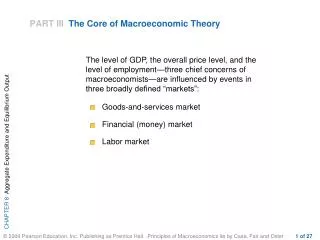
The Core of Macroeconomic Theory. The level of GDP, the overall price level, and the level of employment—three chief concerns of macroeconomists—are influenced by events in three broadly defined “markets”: Goods-and-services market Financial (money) market Labor market.

E N D
The level of GDP, the overall price level, and the level of employment—three chief concerns of macroeconomists—are influenced by events in three broadly defined “markets”: • Goods-and-services market • Financial (money) market • Labor market
FIGURE III.1The Core of Macroeconomic Theory We build up the macroeconomy slowly. In Chapters 8 and 9, we examine the market for goods and services. In Chapters 10 and 11, we examine the money market. Then in Chapter 12, we bring the two markets together, in so doing explaining the links between aggregate output (Y) and the interest rate (r), and derive the aggregate demand curve. In Chapter 13, we introduce the aggregate supply curve and determine the price level (P). We then explain in Chapter 14 how the labor market fits into the macroeconomic picture.
Aggregate Expenditure and Equilibrium Output 10 CHAPTER OUTLINE The Keynesian Theory of Consumption Other Determinants of Consumption Planned Investment (I) The Determination of Equilibrium Output (Income) The Saving/Investment Approach to Equilibrium Adjustment to Equilibrium The Multiplier The Multiplier Equation The Size of the Multiplier in the Real World Looking Ahead Appendix: Deriving the Multiplier Algebraically
aggregate outputThe total quantity of goods and services produced (or supplied) in an economy in a given period. aggregate incomeThe total income received by all factors of production in a given period. In any given period, there is an exact equality between aggregate output (production) and aggregate income. You should be reminded of this fact whenever you encounter the combined term aggregate output (income) (Y). aggregate output (income) (Y)A combined term used to remind you of the exact equality between aggregate output and aggregate income.
The Keynesian Theory of Consumption consumption functionThe relationship between consumption and income. FIGURE 8.1A Consumption Function for a Household A consumption function for an individual household shows the level of consumption at each level of household income.
To explain aggregate spending behavior, economists speculate that an increase in aggregate income in a given period will result in an increase in aggregate consumption in all of the following instances, except: a. When household wealth increases. b. When interest rates rise. c. When households form positive expectations about the future. d. None of the above. In all of the cases above, aggregate consumption will rise.
To explain aggregate spending behavior, economists speculate that an increase in aggregate income in a given period will result in an increase in aggregate consumption in all of the following instances, except: a. When household wealth increases. b. When interest rates rise. c. When households form positive expectations about the future. d. None of the above. In all of the cases above, aggregate consumption will rise.
The Keynesian Theory of Consumption With a straight line consumption curve, we can use the following equation to describe the curve: C = a + bY FIGURE 8.2An Aggregate Consumption Function The aggregate consumption function shows the level of aggregate consumption at each level of aggregate income. The upward slope indicates that higher levels of income lead to higher levels of consumption spending.
The Keynesian Theory of Consumption marginal propensity to consume (MPC) That fraction of a change in income that is consumed, or spent. aggregate saving (S) The part of aggregate income that is not consumed. S ≡Y– C
When aggregate consumption is plotted along a straight line, C = a + bY, an increase in income results in an increase in consumption equal to: a. b. b. b times ΔY. c. a times ΔY. d. a + b.
When aggregate consumption is plotted along a straight line, C = a + bY, an increase in income results in an increase in consumption equal to: a. b. b. b times ΔY. c. a times ΔY. d. a + b.
The Keynesian Theory of Consumption identitySomething that is always true. marginal propensity to save (MPS)That fraction of a change in income that is saved. MPC + MPS≡ 1 Because the MPC and the MPS are important concepts, it may help to review their definitions. The marginal propensity to consume (MPC) is the fraction of an increase in income that is consumed (or the fraction of a decrease in income that comes out of consumption). The marginal propensity to save (MPS) is the fraction of an increase in income that is saved (or the fraction of a decrease in income that comes out of saving).
The Keynesian Theory of Consumption FIGURE 8.3The Aggregate Consumption Function Derived from the Equation C = 100 + .75Y In this simple consumption function, consumption is 100 at an income of zero. As income rises, so does consumption. For every 100 increase in income, consumption rises by 75. The slope of the line is .75.
The Keynesian Theory of Consumption FIGURE 8.4Deriving the Saving Function from the Consumption Function in Figure 8.3 Because S ≡ Y–C, it is easy to derive the saving function from the consumption function. A 45° line drawn from the origin can be used as a convenient tool to compare consumption and income graphically. At Y = 200, consumption is 250. The 45° line shows us that consumption is larger than income by 50. Thus, S ≡ Y–C = 50. At Y = 800, consumption is less than income by 100. Thus, S = 100 when Y = 800.
Fill in the blanks. Where the consumption function is below the 45° line, consumption is ________ than income, and saving is ________. a. more; positive b. more; negative c. less; positive d. less; negative
Fill in the blanks. Where the consumption function is below the 45° line, consumption is ________ than income, and saving is ________. a. more; positive b. more; negative c. less; positive d. less; negative
The Keynesian Theory of Consumption Other Determinants of Consumption The assumption that consumption depends only on income is obviously a simplification. In practice, the decisions of households on how much to consume in a given period are also affected by their wealth, by the interest rate, and by their expectations of the future. Households with higher wealth are likely to spend more, other things being equal, than households with less wealth.
Planned Investment (I) planned investment (I) Those additions to capital stock and inventory that are planned by firms. actual investment The actual amount of investment that takes place; it includes items such as unplanned changes in inventories. FIGURE 8.5The Planned Investment Function For the time being, we will assume that planned investment is fixed. It does not change when income changes, so its graph is a horizontal line.
The Determination of Equilibrium Output (Income) equilibriumOccurs when there is no tendency for change. In the macroeconomic goods market, equilibrium occurs when planned aggregate expenditure is equal to aggregate output. planned aggregate expenditure (AE)The total amount the economy plans to spend in a given period. Equal to consumption plus planned investment: AE≡C + I. Y > C + I aggregate output > planned aggregate expenditure C + I > Yplanned aggregate expenditure > aggregate output
The Determination of Equilibrium Output (Income) FIGURE 8.6Equilibrium Aggregate Output Equilibrium occurs when planned aggregate expenditure and aggregate output are equal. Planned aggregate expenditure is the sum of consumption spending and planned investment spending.
Refer to the figure below. When aggregate output equals $800 billion, which of the following happens? a. Unplanned inventory is rising, and output will tend to rise. b. Unplanned inventory is rising, and output will tend to fall. c. Unplanned inventory is falling, and output will tend to rise. d. Unplanned inventory is falling, and output will tend to fall.
Refer to the figure below. When aggregate output equals $800 billion, which of the following happens? a. Unplanned inventory is rising, and output will tend to rise. b. Unplanned inventory is rising, and output will tend to fall. c. Unplanned inventory is falling, and output will tend to rise. d. Unplanned inventory is falling, and output will tend to fall.
The Determination of Equilibrium Output (Income) The Saving/Investment Approach to Equilibrium Because aggregate income must be saved or spent, by definition, Y ≡ C + S, which is an identity. The equilibrium condition is Y = C + I, but this is not an identity because it does not hold when we are out of equilibrium. By substituting C + S for Y in the equilibrium condition, we can write: C + S = C + I Because we can subtract C from both sides of this equation, we are left with: S = I Thus, only when planned investment equals saving will there be equilibrium.
The Determination of Equilibrium Output (Income) The Saving/Investment Approach to Equilibrium FIGURE 8.7The S = I Approach to Equilibrium Aggregate output is equal to planned aggregate expenditure only when saving equals planned investment (S = I). Saving and planned investment are equal at Y = 500.
The Determination of Equilibrium Output (Income) Adjustment to Equilibrium The adjustment process will continue as long as output (income) is below planned aggregate expenditure. If firms react to unplanned inventory reductions by increasing output, an economy with planned spending greater than output will adjust to equilibrium, with Y higher than before. If planned spending is less than output, there will be unplanned increases in inventories. In this case, firms will respond by reducing output. As output falls, income falls, consumption falls, and so on, until equilibrium is restored, with Y lower than before.
The Multiplier multiplierThe ratio of the change in the equilibrium level of output to a change in some exogenous variable. exogenous variableA variable that is assumed not to depend on the state of the economy—that is, it does not change when the economy changes.
The Multiplier FIGURE 8.8The Multiplier as Seen in the Planned Aggregate Expenditure Diagram At point A, the economy is in equilibrium at Y = 500. When I increases by 25, planned aggregate expenditure is initially greater than aggregate output. As output rises in response, additional consumption is generated, pushing equilibrium output up by a multiple of the initial increase in I. The new equilibrium is found at point B, where Y = 600. Equilibrium output has increased by 100 (600 - 500), or four times the amount of the increase in planned investment.
Refer to the figure below. In this example, the size of the multiplier equals: a. 1.33 b. 25 c. 4 d. 100.
Refer to the figure below. In this example, the size of the multiplier equals: a. 1.33 b. 25 c. 4 d. 100.
The Multiplier The Multiplier Equation Recall that the marginal propensity to save (MPS) is the fraction of a change in income that is saved. It is defined as the change in S (∆S) over the change in income (∆Y): Because DS must be equal to DI for equilibrium to be restored, we can substitute DI for DS and solve: Therefore, It follows that , or
In our simple economy (Y = C + I), when investment rises, equilibrium income will change by: a. b. c. d.
In our simple economy (Y = C + I), when investment rises, equilibrium income will change by: a. b. c. d.
Looking Ahead In this chapter, we took the first step toward understanding how the economy works. We assumed that consumption depends on income, that planned investment is fixed, and that there is equilibrium. We discussed how the economy might adjust back to equilibrium when it is out of equilibrium. We also discussed the effects on equilibrium output from a change in planned investment and derived the multiplier. In the next chapter, we retain these assumptions and add the government to the economy.
multiplier planned aggregate expenditure (AE) planned investment (I) 1. S ≡ Y − C 2. 3. MPC + MPS ≡ 1 4. AE ≡ C + I 5. Equilibrium condition: Y = AE or Y = C + I 6. Saving/investment approach to equilibrium: S = I 7. R E V I E W T E R M S A N D C O N C E P T S actual investment aggregate income aggregate output aggregate output (income) (Y) aggregate saving (S) consumption function equilibrium exogenous variable identity marginal propensity to consume (MPC) marginal propensity to save (MPS)