Download
1 / 19
190 likes | 320 Views
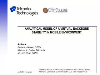
ANALYTICAL MODEL OF A VIRTUAL BACKBONE STABILITY IN MOBILE ENVIRONMENT. General Concept: Reliable Server Pooling (RSP). Goal: Providing naming service to clients that need uninterrupted access to servers Focus: Scalable and survivable architecture for ad hoc networks. peer discovery.

E N D
ANALYTICAL MODEL OF A VIRTUAL BACKBONE STABILITY IN MOBILE ENVIRONMENT
General Concept: Reliable Server Pooling (RSP) • Goal: Providing naming service to clients that need uninterrupted access to servers • Focus: Scalable and survivable architecture for ad hoc networks peer discovery associate, request, PE failure Pool Users (PUs) Name Servers (NSs) advertise associate, register, I am alive Pool 1: PE11, PE12, … Pool N: PEN1, PEN2, … Pool Elements (PEs)
RSP Scope NS2 (PE2’s home) (2) PE2 fail (5) PU1 NS1 (PU1’s home) (3) (1) (4) PE1 PE2 (6) PE2 is dereg’ed Pool
Router R Border Router BR ENRP2' ENRP2 ENRP1 PU PU PU PU PU PU PU1 PE4 PE2 PE3 PE5 PE1 BR RSP across multiple domains Name Server(Endpoint Name Resolution Protocol) ENRP Pool: Elements Users PE PU ENRP Backbone Network R Pool: PE1, PE2, PE3, PE4, PE5 R R hub R • ENRP1 knows only PE1 and PE2 • both quickly made available to PU1 • PE1 can fail over from PE1 to PE2 • ENRP1 may or may not contact ENRP2 • if YES, then PE3, PE4, and PE5 • become available to PU1 after delay ENRP PE PU R D1 BR (5) D2 (4) (3) (1) (2) (6) (7) (8)
RSP across multiple domains • Experiments show that a single flat namespace causes problems • signaling overhead due to hunting for Home NS and/or advertisements • difficulty in synchronizing among multiple NSs • Investigating multiple domains and local name spaces • features • one logical NS per domain (primary plus backups) • pools may span multiple domains and local name spaces • NS keeps only partial membership information for a given pool • advantages • limited traffic: home hunt, NS advertisements, PE heartbeats, etc... • no need to synchronize NSs • quick response within local domain • issues • load balancing among PEs may not be optimum within domain • new procedure needed for querying NSs in other domains to get a complete pool-membership information • protocols need to be redesigned • expect to further reduce the signaling overhead
RSP over Virtual Backbone • Main focus: Registration and discovery services for PEs/PUs • Developed new architecture and protocols for RSP • Novel scheme is calledDynamic Survivable Resource Pooling (DSRP) • DSRP implements RSP over virtual backbone for ad hoc networks • DSRP architecture is (practically) infrastructure-less • No fixed infrastructure; system fully distributed • Naming system deployed on dynamically assigned VB nodes • backbone nodes serve as dynamic Name Servers • NSs form an overlay of nodes as a connected dominating set (CDS) • VB is highly survivable • Main Features of DSRP • Reorganization in response to mobility, failures, and partitioning • Fast response time if local name resolution possible • Load balancing of pool elements provided by NSs or pool users • Scalability when the network size grows
Analytical Model of DSRP • Motivation • Only simulations available for single-PE discovery over VB • Approach • Main end-user metric: • What is the expected delay to get service request resolved? • Steps • probability of a PE/PU (not) having an operational PNS • stability of NS, i.e., expected time for NS to leave the backbone • expected delay for PE/PU to find new PNS when the previous one becomes unavailable • Base model • We adapted the discrete-time random walk model proposed by Y. Tseng et al., “On Route Lifetime in Multihop Mobile Ad Hoc Networks” • Dynamics of nodes and VB driven by random node movement • Probabilistic link creation/failure models
y (-1,4) (1,3) (1,-4) <2,0> Area covered by MANET (0,4) (0,3) (2,2) (-2,4) x Available Link state nav=2 (-1,3) (3,1) (-3,4) (1,2) Total number of layers ntot=9 (4,0) (2,1) (-4,4) (-2,3) (0,2) (3,0) (-1,2) (-3,3) (1,1) MN2 (2,0) (-2,2) (-4,3) (0,1) (4,-1) (1,0) (-3,2) (-1,1) (3,-1) MN1 Unavailable Link state n=4 <-4,4> (2,-1) (-2,1) (0,0) (-4,2) (4,-2) (-1,0) (-3,1) (1,-1) (3,-2) <2,0> <4,-4> MN4 (-2,0) (-4,1) (4,-3) (0,-1) (2,-2) MN3 (-3,0) (-1,-1) (3,-3) (1,-2) (-4,0) (-2,-1) (2,-3) (0,-2) (4,-4) (-3,-1) (-1,-2) (1,-3) (3,-4) (0,-3) (-2,-2) (2,-4) (-1,-3) (0,-4)
(0,1) (x,y+1) <x,y> D1 D1 (1,0) (-1,1) (x+1,y) (x-1,y+1) D6 D6 (x,y) (0,0) D2 D2 <x,y> MN1 D5 D5 MN2 D3 (x-1,y) D3 (-1,0) (1,-1) <x+1,y> (x+1,y-1) D4 D4 (x,y-1) (0,-1) Random Walk Model and Link State Changes Figure Example link state changes • The probability distribution for a wireless link to switch from state <x,y> to state <x’,y’> after one time unit
State Transition Diagram and our modifications nav=5 ntot NOTE: taken from the Tseng’s paper • They consider only available links • Extending the number of layers to cover all area (all available and unavailable links) • Bouncing back from the highest layer • M represents state transition matrix obtained using the state transition diagram
Analytical Model • VB behavior with respect to link changes • VB nodes are determined dynamically when the network topology changes • Preference given to a node with the highest degree, i.e., the number of available links • We approximate this behavior by considering the threshold number of available links • We are interested in expected times to cross the threshold • Mi,jrepresents the probability to transit from the ith state to jth state • Suppose that a wireless link is in state i at initial. Pa(i) and Pu(i) denote the probabilities that the link will be available and unavailable in the next time unit, respectively • j= 0, 1, 2, …., sarepresent available link states • j= sa+1, sa+2, …., sTrepresent unavailable link states
Analytical Model • Assume there are N mobile nodes in the network • Consider only a particular node. There are K=N-1 possible bidirectional links from this node to all other nodes • Assume k available links for this node, there are Ku=K-k unavailable links • Let Pdap(k,l) denote the probability that l of k available links will disappear and Pap(Ku,l+1) denote the probability that l+1 of Ku unavailable links will appear in one time unit • If we use the steady state values of the state transition matrix Mi,j , then Pa(i) will be same for all inner link states i and Pu(i) will be same for all outer link states i
Analytical Model • Then Equations 3 and 4 will be simplified as follows: • Given that there are k available links, Pk,k+1denotes the probability that there will be k+1 available links in the next time unit • If we generalize the above formula for Pk,k+hwhere h can be negative or positive (all possible number of link changes)
0 k-h k-1 k k+1 k+h K Pk-h,K P0,K Pk-1,K P0,k+h Pk,K Pk+h,K P0,0 PK,k+h PK,k Pk+h,0 PK,k-1 PK,0 PK,k-h • A new Markov chain obtained using the stationary distribution of the state transition matrix M. Here, a state represents the number of available links for a node • P is the corresponding state transition matrix
Number of available links dthr d0 m 0 1 2 3 m-1 m+1 4 Time steps Analytical Model πkdenotes the steady state probabilities of the P matrix. Let a random variable Z denote the number of link changes in one time unit. The probability distribution of Z can be calculated as follow: Z1, Z2, …, Zm represent the link changes for 1st, 2nd, …, mthsteps and Sm represents the net link change until the mth step
0 k-h k-1 k k+1 dthr First Passage Time Analysis • The number of transitions going from one state to another for the first time • We combined states equal to or greater than dthr into a single state dthr • We modified the transition probabilities: only the dashed lines are modified • The expected first times going from k to dthr, given that there are k (k < dthr) available links at initial, using the above Markov chain 1
Numerical Results • N: number of nodes, ntot: total number of layers, nav: number of layers representing available links • ntot determines the size of the geographic area for the fixed cell size • For numerical results, N=106, nav=5, d0=0 and dthr varied • Network types in terms of its density: sparsest (ntot=40), sparse (ntot=30), typical (ntot=20), dense (ntot=15), and densest (ntot=10)
Conclusion and Future Work • The mobility part of DSRP has been modeled analytically Future Work: • Finding one unit time for different cell size and mobile node speed distributions • Combining this analysis with backbone formation and maintenance algorithms to find the expected time that an NS will remain an NS and the expected time that a non-NS will be an NS • Finally, developing an analytical model for DSRP using the above expected times together with a service discovery model • Application to other schemes depending on link stability • Routing • Bandwidth-estimation algorithms
5 5 5 5 Part I: Backbone Formation and Maintenance White – Undecided nodes Black – VB nodes (decided) Green – non-VB nodes (decided) 21 2 41 4 76 7 1 1 51 3 31 6 6