Download
1 / 19
190 likes | 302 Views
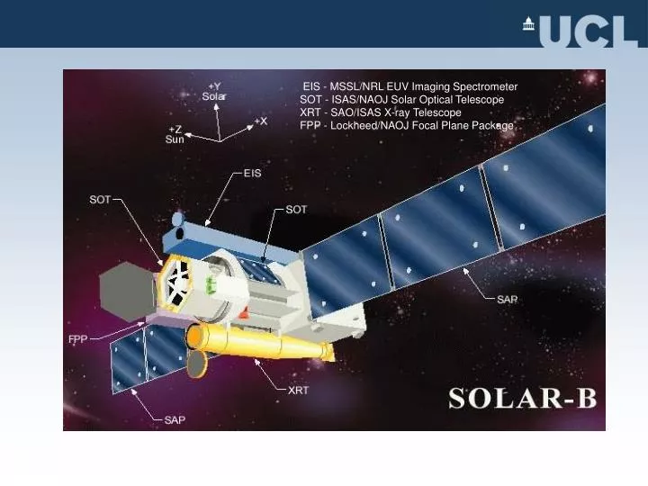
EIS - MSSL/NRL EUV Imaging Spectrometer SOT - ISAS/NAOJ Solar Optical Telescope XRT - SAO/ISAS X-ray Telescope FPP - Lockheed/NAOJ Focal Plane Package. Mission Characteristics. Launch date: August 2006 Launch vehicle: ISAS MV Mission lifetime: 3 years. Orbit: Polar, sun synchronous

E N D
EIS - MSSL/NRL EUV Imaging Spectrometer SOT - ISAS/NAOJ Solar Optical Telescope XRT - SAO/ISAS X-ray Telescope FPP - Lockheed/NAOJ Focal Plane Package
Mission Characteristics • Launch date: August 2006 • Launch vehicle: ISAS MV • Mission lifetime: 3 years • Orbit: Polar, sun synchronous • Inclination: 97.9 degrees • Altitude: 600 km. • Mass: 900 kg
EIS - Instrument Features • Large Effective Area in two EUV bands: 170-210 Å and 250-290 Å • Multi-layer Mirror (15 cm dia ) and Grating; both with optimised Mo/Si Coatings • CCD camera; Two 2048 x 1024 high QE back illuminated CCDs • Spatial resolution: 1 arcsec pixels/2 arcsec resolution • Line spectroscopy with ~ 25 km/s pixel sampling • Field of View: • Raster: 6 arcmin×8.5 arcmin; • FOV centre moveable E – W by ± 15 arcmin • Wide temperature coverage: log T = 4.7, 5.4, 6.0 - 7.3 K • Simultaneous observation of up to 25 lines
EIS Optical Diagram Primary Mirror 1939 mm Slit Exchange Mechanism Shutter Entrance Filter CCDs Filter 1000 mm 1440 mm Concave Grating Primary Mirror Entrance Filter CCD Camera Front Baffle Grating
Dual CCD Camera Grating Primary Mirror EIS Instrument Completed Filter Holder Installed Entrance Filter Holder Installation of Key Subsystems in Structure
w Observables • Observation of single lines • Line intensity and profile • Line shift () → Doppler motion • Line width (w) and temperature → Nonthermal motion • Observation of line pair ratios • Temperature • Density • Observation of multiple lines • Differential emission measure
1024 pixels Emission Lines on EIS CCDs
Slit and Slot Interchange • Four slit/slot selections available • EUV line spectroscopy - Slits - 1 arcsec 512 arcsec slit - best spectral resolution - 2 arcsec 512 arcsec slit - higher throughput • EUV Imaging – Slots • Overlappogram; velocity information overlapped • 40 arcsec 512 arcsec slot - imaging with little overlap • 250 arcsec 512 arcsec slot - detecting transient events
Shift of FOV center with coarse-mirror motion Maximum FOV for raster observation 360 900 900 512 512 512 Raster-scan range 250 slot 40 slot EIS Slit EIS Field-of-View (FOV)
Detected photons per 11 area of the sun per 1 sec exposure. AR: active region EIS Sensitivity
Expected Accuracy of Velocity Flare line Bright AR line Photons (11 area)-1 sec-1 Photons (11 area)-1 (10sec)-1 Doppler velocity Line width Number of detected photons
Norikura coronagraph observations of all three of these parameters Processed Science Data Products • Intensity Maps (Te, ne): – images of region being rastered from the zeroth moments of strongest spectral lines • Doppler Shift Maps (Bulk Velocity): – images of region being rastered from first moments of the strongest spectral lines • Line Width Maps (NT Velocity): – images of region being rastered from second moments of the strongest spectral lines
The first 3 months…. • Flare trigger and dynamics:Spatial determination of evaporation and turbulence in a flare • Active region heating:Spatial determination of the velocity field in active region loops • Coronal Hole Boundaries:Measurement of intensity and velocity field at a coronal hole boundary • Quiet Sun Brightenings:Determination of the relationship between different categories of quiet Sun events.
Active Regions • connect the photospheric velocity field to the signatures of coronal heating. This will allow us to determine the dominant heating mechanism in active regions, and will be extended to other coronal brightenings. • search for evidence of waves in loops and make use of observations for coronal seismology • study dynamic phenomena within active region loops.
Quiet Sun • link quiet Sun brightenings and explosive events to the magnetic field changes in the network and inter-network to understand the origin of these events. • determine the variation of explosive events and blinkers with temperature. • Search for evidence of reconnection and flows at junctions between open and closed magnetic field at coronal hole boundaries. • Determine the impact of quiet Sun events on larger scale structures within the corona. • Determine physical size scales using density diagnostics.
Solar Flares • determine the source and location of flaring and identify the source of energy for flares. EIS will measure the velocity fields and observe coronal structures with temperature information. Hence will allow us to address the trigger mechanism. • detection of reconnection inflows, outflows and the associated turbulence which play the pivotal role in flare particle acceleration.
Coronal Mass Ejections • determine the location of dimming (and the subsequent velocities) in various magnetic configurations allowing us to determine the magnetic environment that leads to a coronal mass ejection. • The situations to be studied include filaments, flaring active regions and trans-equatorial loops.
Large Scale Structures • determine the temperature and velocity structure in a coronal streamer • determine the velocity field and temperature change of a trans-equatorial loop, and search for evidence of large-scale reconnection. • Using a low-latitude coronal hole, search for evidence of the fast solar wind.
Information is maintained on our website; http://www.mssl.ucl.ac.uk/www_solar/solarB/ The EIS science planning guide shows details of the 3 month plan studies including line choices, which slit/slot, FOV etc. The planning software will be released into SSW in the autumn. Quicklook software etc. is already in SSW. Details are on the website. The next solar-B science meeting will be in Kyoto in November.