Image Enhancement in Fourier Transform

2. Image Enhancement in Fourier Transform

10. Filtering in the Frequency Domain • A binary image is created which contains a white rectangle at its center. After taking its fast • Fourier transform in 2D (using fft2 matlab® image processing toolbox function, the Fourier • spectrum is displayed in a window.

11. Filtering in the Frequency Domain • clear all • close all • clc • % • % Form a white rectangle of size 5x5 superimposed on a black • % background of size 30x30 • N = 30; • f = zeros(N,N); • f(13:17,13:17) = 1; • figure, imshow(f, 'notruesize'); • % • % Take 2D fast Fourier Transform • F = fft2(f, 256, 256); • % • % Show the resulting Fourier Spectrum after • % logarithmically compressing the dynamic range • figure, imshow(log(abs(F)+1), [-1 5]); • % • % Shift the Fourier Spectrum to the center of the • % uv-coordinates • G = fftshift(F); • figure, imshow(log(abs(G)+1), [-1 5]);

12. Image of a 5x5 white rectangle on a black background of size 30x30 Fourier Spectrum Centered Fourier Spectrum

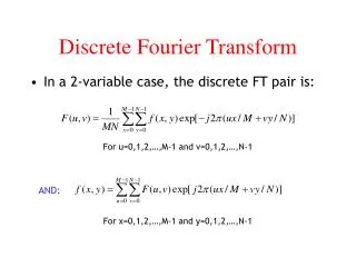
13. Steps to Take FFT • Once in the frequency domain, the image can be filtered. The basic steps involved in majority of the frequency domain filtering techniques are: • Pre-process the image f (x, y) . • Compute F(u, v) , the Discrete Fourier Transform (DFT) of the image. • Multiply F(u, v) by a filter function H(u, v) • Compute the inverse DFT of the resulting image. • Obtain the real part (or magnitude) of the result of step 4. • Post-process the resulting image g( x, y) .

14. Smoothing Frequency Domain Filters • We cover two different types of smoothing filters in this section. An ideal low pass filter which represents the category of very sharp/crisp filters, and the Butterworth low pass filter, which belongs to the category of smooth filters. • The variation in the filter values is very sharp in case of ideal filters and relatively smooth in case of Butterworth filters. There are other types of smoothing filters as well, e.g. a Gaussian filter, where the variations are even smoother than the Butterworth filter. • The main aim of all these filters is to smooth out the discontinuities in the original image. • Large “size” frequency domain filters give rise to less smoothing, while small “size” filters in the frequency domain result in more smoothing and sometimes blurriness.

15. Ideal Low Pass Filter • We design first an ideal low pass filter and then apply it to an image. • close all • clear all • clc • % Load a gray scale image • I=imread('cameraman.tif'); • % • % Show the image • figure;imshow(I,[]); • % • % Take the 2D Fast Fourier Transform • FI = fft2(I);

16. Ideal Low Pass Filter • % • % Shift the DC component to the center • SFI = fftshift(FI); • % • % Use logarithmic compression of dynamic range • % and display the image • figure;imshow(log(1+abs(SFI)),[]); • % • % Find out the size of the image • [n,m] = size(SFI); • % • % Initialize an n x m matrix • h = zeros(n,m);

17. Ideal Low Pass Filter • % Define the frequency cutoff • d0 = 0.005*n*m; • for k = 1:n, • for l = 1:m, • i1 = (n/2) - k; • j1 = (m/2) - l; • d = i1*i1 + j1*j1; • if d < d0 • h(k,l) = 1; • end • end • end

18. Ideal Low Pass Filter • % Show the filter • figure;imshow(h,[]); • figure; mesh(h(1:5:end,1:5:end)); • figure; surf(h(1:5:end,1:5:end)); • % • % Find out the filtered response and display it • ASFI = h.*SFI; • figure;imshow(log(1+abs(ASFI)),[]); • % • % Calculate the inverse Fourier transform and • % display the filtered response • IASFI = ifft2(ASFI); • figure;imshow(abs(IASFI),[]);

19. Ideal Low Pass Filter

20. Butterworth Low Pass Filter • As mentioned earlier, a Butterworth filter is not as abrupt as an ideal filter, the variations in the filters values are kept smooth with the help of the working parameters of the filter.

21. Butterworth Low Pass Filter • h = ones(n,m); • % • % Define the frequency cutoff • d0 = 0.01*n*m; • for k = 1:n, • for l = 1:m, • i1 = (n/2) - k; • j1 = (m/2) - l; • d = i1*i1 + j1*j1; • h(k,l) = 1 / (1+(d/d0)^2); • end • end

22. Butterworth Low Pass Filter