Molecular Dynamics Simulations An Introduction N. Gautham

1. Molecular Dynamics Simulations An Introduction N. Gautham Department of Crystallography and Biophysics University of Madras, Guindy Campus Chennai 600 025 gautham@unom.ac.in

2. Molecular Dynamics • Definitions, Motivations • Force fields • Algorithms and computations • Water and Solvent

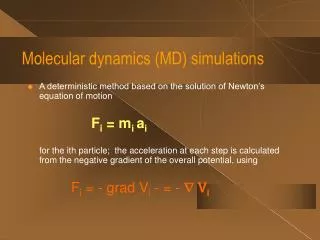
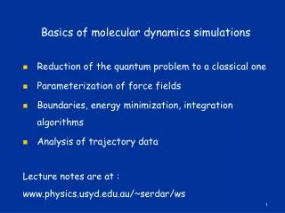
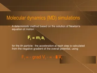
3. Molecular dynamics - Introduction • Molecular dynamics (MD) is a computer simulation technique where the time evolution of a set of interacting atoms is followed by integrating their equations of motion. • We follow the laws of classical mechanics, and most notably Newton's law:

4. Molecular dynamics - Introduction • Given an initial set of positions and velocities, the subsequent time evolution is in principle completely determined. • Atoms and molecules will ‘move’ in the computer, bumping into each other, vibrating about a mean position (if constrained), or wandering around (if the system is fluid), oscillating in waves in concert with their neighbours, perhaps evaporating away from the system if there is a free surface, and so on, in a way similar to what real atoms and molecules would do.

5. Molecular dynamics -Motivation • The computer experiment. • In a computer experiment, a model is still provided by theorists, but the calculations are carried out by the machine by following a recipe (the algorithm, implemented in a suitable programming language). • In this way, complexity can be introduced (with caution!) and more realistic systems can be investigated, opening a road towards a better understanding of real experiments.

6. Molecular dynamics -Motivation • The computer calculates a trajectory of the system • 6N-dimensional phase space (3N positions and 3N momenta). • A trajectory obtained by molecular dynamics provides a set of conformations of the molecule, • They are accessible without any great expenditure of energy (e.g. breaking bonds) • MD also used as an efficient tool for optimisation of structures (simulated annealing).

7. Molecular dynamics - Motivation • MD allows to study the dynamics of large macromolecules • Dynamical events control processes which affect functional properties of the biomolecule (e.g. protein folding). • Drug design is used in the pharmaceutical industry to test properties of a molecule at the computer without the need to synthesize it.

8. Molecular dynamics - Introduction • In molecular dynamics, atoms interact with each other. • These interactions are due to forces which act upon every atom, and which originate from all other atoms • Atoms move under the action of these instantaneous forces. • As the atoms move, their relative positions change and forces change as well.

9. Molecular dynamics – Time Limitations • Typical MD simulations are performed on systems containing thousandsof atoms • Simulation times range from a few picoseconds to hundreds of nanoseconds. • A simulation is reliable when the simulation time is much longer than the relaxation time of the quantities we are interested in.

10. Molecular dynamics – The model

11. Molecular dynamics – Force Fields • Epot = SVbond + SVang + SVtorsion +SVvdW + SVele+ … • Other terms (the ‘…’) • Planarity constraints • Hydrogen bonding potentials • Interaction terms (between different types of motion e.g. bond length stretch – bond angle bend)

12. Molecular dynamics – Force Fields • The potential as specified by the above has an infinite range. • In practical applications, it is customary to establish a cutoff radius Rc and disregard the interactionsbetween atoms separated by more than Rc

13. Molecular dynamics – Force Fields • What should we do at the boundaries of our simulated system? • If nothing special is done, atoms near the boundary would have less neighbours than atoms inside. • This causes surface effects in the simulation to be much more important than they are in the real system.

14. Molecular dynamics – Force Fields • A solution to this problem is to use periodic boundary conditions (PBC). • We use the minimum image criterion: among all possible images of a particle j, select only the closest.

15. Molecular dynamics – Algorithms • The engine of a molecular dynamics program is its time integration algorithm. • Time integration algorithms are based on finite difference methods, where time is discretized on a finite grid, the time stept being the distance between consecutive points on the grid • Knowing the positions and some of their time derivatives at time t, the integration scheme gives the same quantities at a later time t+t • By iterating the procedure, the time evolution of the system can be followed for long times.

16. Molecular dynamics – Algorithms • These schemes are approximate and there are errors associated with them • Truncation errors are related to the accuracy of the finite difference method with respect to the true solution. These errors are intrinsic to the algorithm. • Round-off errors are related to errors associated to a particular implementation of the algorithm. For instance, to the finite number of digits used in computer arithmetic. • Both errors can be reduced by decreasing t

17. Molecular dynamics – Algorithms • Two popular integration methods for MD calculations are the Verlet algorithm and predictor-corrector algorithms • The most commonly used time integration algorithm is the Verlet algorithm

18. Molecular dynamics – Algorithms • The predictor-corrector algorithm consists of three steps • Step 1:Predictor. From the positions and their time derivatives at time t, one ‘predicts’ the same quantities at time t+t by means of a Taylor expansion. Among these quantities are, of course, accelerations ‘a’ • Step 2:Force evaluation. The force is computed by taking the gradient of the potential at the predicted positions.

19. Molecular dynamics – Algorithms • Step 2 (contd.):The difference between the resulting acceleration and the predicted acceleration constitutes an ‘error signal • Step 3:Corrector. This error signal is used to ‘correct’ positions and their derivatives. All the corrections are proportional to the error signal, the coefficient of proportionality being determined to maximize the stability of the algorithm.

20. Molecular dynamics – Algorithms • To start the simulationwe have tocreate a set of initial positions and velocities for the atoms in the molecule • The initial positions usually correspond to a known structure (from X-ray or NMR structures, or predicted models) • The initial velocities are assigned taking them from a Maxwell distribution at a certain temperature T • Another possibility is to take the initial positions and velocities to be the final positions and velocities of a previous MD run

21. Molecular dynamics – Water and solvent • The molecule is positioned in a box of size approximately twice the largest dimension of the molecule • The molecule is solvated by adding water (or other solvent molecules) at random positions in the box – no two atoms can be touching each other

22. Molecular dynamics – Algorithms • Every time the state of the system changes (e.g. when we start the simulation) the system will be out of equilibrium for a while • We usually want equilibrium to be reached before starting performing measurements on the system • A physical quantity A generally approaches its equilibrium value exponentially with time:  •  may be a few hundred time steps, allowing us to see A(t) converge to Ao

23. Molecular dynamics – Analyses • The simplest way of analyzing the system during (or after) its dynamic motion islooking at it. • One can assign a radius to the atoms, represent the atoms as balls having that radius, and have a computer program construct a ‘photograph’ of the system. • We may also colour the atoms according to its properties (charge, displacement, ‘temperature’…)

24. Molecular dynamics – Analyses • We also can measure instantaneous and time averages of various physically important quantities • To measure time averages: If the instantaneous values of some property A at time t is • then its average is • where NT is the number of steps in the trajectory

25. Molecular dynamics – Analyses Analyses using ‘trajectories’

26. Molecular dynamics – Analyses

27. Molecular dynamics – Analyses

28. Molecular dynamics – Analyses

29. Molecular dynamics – Analyses

30. Molecular dynamics – Analyses

31. Molecular dynamics – Analyses

32. Molecular dynamics – Optimization tool • Molecular Dynamics may also be used as an optimization tool • Traditional (optimization) minimization techniques (steepest descent, conjugate gradient, etc.) do not normally overcome energy barriers and tend to fall into the nearest local minimum Global minimum energy Conformational space

33. Molecular dynamics – Optimization tool • Temperature in a molecular dynamics calculation provides a way to fly over the barriers • States with energy E are visited with a probability exp(-E/kBT) • By decreasing T slowly to 0, there is a good chance that the system will be able to pick up the best minimum and land into it • This is the simulated annealing protocol, where the system is equilibrated at a certain (high) temperature and then slowly cooled down to T=0

34. Molecular dynamics – Optimization tool Trajectory energy Conformational space

35. Molecular dynamics – Other Methods • We have discussed so far the standard molecular dynamics scheme, based on the time integration of Newton's equations and leading to the conservation of the total energy. • In the statistical mechanics parlance, these simulations are performed in the microcanonical ensemble, or NVE ensemble • The number of particles, the volume and the energy are constant quantities.

36. Molecular dynamics – Other Methods • There are other important alternatives to the NVE ensemble • A scheme for simulations in the isoenthalpic-isobaric ensemble (NPH) has been developed • The volume V of the box is variable. The enthalpy H=(E+PV) is a conserved quantity. • Another very important ensemble is the canonical ensemble (NVT). • The temperature is kept constant

37. Molecular mechanics – References • Molecular Modelling • A.R. Leach (2001) Prentice Hall. • Understanding Molecular Simulation • D. Frenkel and B. Smit (1996) Academic Press • Molecular Dynamics Simulation • J.M. Haile (1992) John Wiley • http://www.fisica.uniud.it/~ercolessi/md/md/md.html