Download
1 / 12
120 likes | 228 Views
LECTURE 16: EM AND SIMPLE REGRESSION. Objectives: Feature and Model Space Adaptation General Adaptation Framework Expectation Maximization Simple Linear Regression

E N D
LECTURE 16: EM AND SIMPLE REGRESSION • Objectives:Feature and Model Space AdaptationGeneral Adaptation FrameworkExpectation MaximizationSimple Linear Regression • Resources:ECE 8463: Adaptation ECE 8443: Expectation MaximizationWiki: Expectation MaximizationWiki: Linear RegressionMIT: Linear Regression • URL: .../publications/courses/ece_8423/lectures/current/lecture_16.ppt • MP3: .../publications/courses/ece_8423/lectures/current/lecture_16.mp3
Revisiting the Adaptation Problem • Previously, we have focused on adaptionstrategies that involve time series data(e.g., samples of a signal). However, analternative view of this problem is in termsof models and features. • New data can be in the form of samples of a time series or new feature vectors. The former is more common in time series analysis; the latter ismore common in pattern recognition applications. • The reference model is typically derived from extensive amounts of data (e.g., tens of thousands of hours of voice) and uses off-line techniques to estimate the parameters of the model. • The amount of new data is often orders of magnitude smaller (e.g., minutes of voice), and comes from an environment that is significantly different than the reference data. • The reference model normally consists of a large number of parameters, more than can be reliably estimated from only a small amount of new data. • Hence, the adaptation problem revolves around the question of how best we can modify the reference model to better match the new data. CommonSpace Reference New Data
Adaptation Strategies • Possible parameter adaptation strategies: • Normalize the reference model and the newdata to a common space; • Transform the new data into the referencedata space (or alternately transform the referencedata into the new data space); • Reestimate the model parameters by pooling allthe data. • The latter approach is not often practical for two reasons: (1) the computational complexity of the reestimation process is significant, and would typically have to be performed off-line; (2) the new data would be dwarfed by the amount of old data. • Therefore, in this treatment, we will consider the problem of transforming the model to match the statistics of the new data. • Since the amount of new data is small, the number of parameters associated with this transformation must be small (much less than the original model). • We would also prefer this adaptation process to run close to real-time or online – meaning the new model parameters are available shortly after the new data arrives (rather than waiting overnight for the parameter updates.)
MAP vs. MLLR • There are two basic types of adaptation: • Maximum A Priori (MAP): choosing an estimate that maximizes the posterior probability (consistent with the observed data and prior information). • Maximum Likelihood Linear Regression (MLLR): using a maximum likelihood approach to estimate the parameters of a transformation of the feature vectors or model parameters. • To understand either of these approaches, we need to introduce several new analysis and modeling tools. Two of the most important and basic are: • Expectation Maximization Theorem: describes a technique for guaranteeing that our new parameter estimates are “better” than the previous estimates. • Maximum Likelihood Linear Regression: describes a statistical approach to fitting a model, typically a line or regression function, to the data. • In contrast to techniques that minimize the mean square error (e.g., LMS), our goal here will be to produce a model that is better than the previous model. This is, in general, a complicated question that depends on how you define “better.” We will focus on a simple, generative approach, that estimates the probability the training data could have been generated from the model. • A more thorough treatment of such issues is the focus of our Pattern Recognition course.
Expectation Maximization – Synopsis • Expectation maximization (EM) is an approach that is used in many ways to find maximum likelihood estimates of parameters in probabilistic models. • EM is an iterative optimization method to estimate some unknown parameters given measurement data. Used in a variety of contexts to estimate missing data or discover hidden variables. • The intuition behind EM is an old one: alternate between estimating the unknowns and the hidden variables. This idea has been around for a long time. However, in 1977, Dempster, et al., proved convergence and explained the relationship to maximum likelihood estimation. • EM alternates between performing an expectation (E) step, which computes an expectation of the likelihood by including the latent variables as if they were observed, and a maximization (M) step, which computes the maximum likelihood estimates of the parameters by maximizing the expected likelihood found on the E step. The parameters found on the M step are then used to begin another E step, and the process is repeated. • This approach is the cornerstone of important algorithms such as hidden Markov modeling and discriminative training, and has been applied to fields including human language technology and image processing.
Special Case of Jensen’s Inequality • Lemma: If p(x) and q(x) are two discrete probability distributions, then: • with equality if and only if p(x) = q(x) for all x. • Proof: • The last step follows because probability distributions sum (or integrate) to 1. • Note: Jensen’s inequality relates the value of a convex function of an integral to the integral of the convex function and is used extensively in information theory.
The EM Theorem Theorem: If then . Proof: Let y denote observable data. Let be the probability distribution of y under some model whose parameters are denoted by .Let be the corresponding distribution under a different setting .Our goal is to prove that y is more likely under than .Let t denote some hidden, or latent, parameters that are governed by the values of . Because is a probability distribution that sums to 1, we can write: Because we can exploit the dependence of y on t and using well-known properties of a conditional probability distribution.
Proof Of The EM Theorem We can multiple each term by “1”: where the inequality follows from our lemma. Explanation: What exactly have we shown? If the last quantity is greater than zero, then the new model will be better than the old model. This suggests a strategy for finding the new parameters, – choose them to make the last quantity positive!
Discussion • If we start with the parameter setting , and find a parameter setting for which our inequality holds, then the observed data, y, will be more probable under than . • The name Expectation Maximization comes about because we take the expectation of with respect to the old distribution and then maximize the expectation as a function of the argument . • Critical to the success of the algorithm is the choice of the proper intermediate variable, t, that will allow finding the maximum of the expectation of . • Perhaps the most prominent use of the EM algorithm in pattern recognition is to derive the Baum-Welch reestimation equations for a hidden Markov model. • Many other reestimation algorithms have been derived using this approach.
Least Squares Linear Regression • Suppose we are given a sequence of observations: • We want to estimate a function that predicts Y as afunction of X: • The most obvious way to do this would be to minimize themean-square error: • To find the optimal values, differentiate with respect to each parameter: • Let’s introduce some common statistical quantities to simplify our equations: Y x x x x x x X
Solution and Generalization • We can solve these equations for 0 and 1: • What are the strengths and weaknesses of this approach?(Hints: uniform weighting, a priori information) • Generalization (Normal Equation): Y x x x x x x X
Summary • Introduced a general statistical framework for adaptation. • Discussed two general approaches: MAP and MLLR. • Introduced two tools we will use: EM and linear regression. • Derived the equations for estimation of the parameters of the linear regression model using minimum mean-square error. • Next: introduce a probabilistic view of linear regression and derive an estimation procedure that maximizes the likelihood. • Also, introduce MAP adaptation.