Download
1 / 25
250 likes | 425 Views
AGEC 340 – International Economic Development Course slides for week 11 (March 23-25) Demand, supply and market prices*. Where do prices come from?. * If you are following the textbook, this is chapte r 15. Markets & Trade Where do prices come from?.

E N D
AGEC 340 – International Economic DevelopmentCourse slides for week 11 (March 23-25)Demand, supply and market prices* Where do prices come from? * If you are following the textbook, this is chapter 15.
Markets & TradeWhere do prices come from? • So far we’ve looked at development from an individual’s point of view, taking prices as given… but where do prices come from? • What (or who) is ‘the market’? • Econ explains prices in terms of supply & demand • we saw consumer demand in week 3: • Demand is consumers’ willingness and ability to pay • we’ve seen producers’ supply in weeks 6-9: • Supply is producers’ willingness and ability to sell
Where does a supply curve come from? Supply response comes from producers adjusting their production levels along IRCs & PPFs: Qty. of corn (bu/acre) Qty. of corn (bu/acre) To get more corn, use more labor and grow less beans Qty. of labor (hours/acre) Qty. of beans (bushels/acre)
Suppliers’ position along these curves is determined by relative prices Qty. of corn (bu/acre) Qty. of corn (bu/acre) slope of isoprofit line= Plabor/Pcorn slope of the iso-revenue line = -Pbeans/Pcorn Qty. of labor (hours/acre) Qty. of beans (bushels/acre)
When corn prices rise, producers use more inputs. Qty. of corn (bu/acre) a higher Pcorn means a flatter isoprofit line more corn more labor Qty. of labor (hours/acre)
When corn prices rise, producers make less of others goods. Qty. of corn (bu/acre) a higher Pcorn means a flatter iso-revenue line more corn less beans Qty. of beans (bushels/acre)
So, for each individual producer, at every price a specific quantity will be produced... Price ($/lb) 0.75 Quantity Produced (lbs/yr) 10
...and as prices rise a higher quantity will be produced... Price ($/lb) 1.00 0.75 Quantity Produced (lbs/yr) 10 15
…the slope of this curve depends on the slopes of the IRCs and PPFs... Price ($/lb) 1.25 1.00 0.75 Quantity Produced (lbs/yr) 10 15 17
and so the “supply curve” always slopes upward: Price ($/lb) 1.25 1.00 When price changes, producers move along their supply curve 0.75 Quantity Produced (lbs/yr) 10 15 17
Adding up all producers together, we have a market supply curve: Price ($/lb) each producer’s production is added horizontally 1.25 1.00 0.75 Quantity Produced (thousands of tons/yr) 10 15 17 Note the new scale!
Similarly, we can draw a demand curvefor each individual consumer... Price ($/lb) 1.25 When price changes, consumers move along their demand curve 1.00 0.75 Quantity Consumed (lbs/yr) 10 15 17
…and then add up all consumers togetherwe get the market demand curve: Price ($/lb) each consumer’s demand is added horizontally 1.25 1.00 0.75 Quantity Consumed (thousands of tons/yr) 10 15 17 Again we change scale to show total market demand
And we can put the two together in a “supply-demand diagram” Price ($/lb) 1.25 All producers’ market supply curve 1.00 0.75 All consumers’ market demand curve Quantity (thousands of tons/yr) 10 15 17
…so what price do we expect to observe? Price ($/lb) 1.25 market supply 1.00 0.75 market demand Quantity (thousands of tons/yr) 10 15 17
We expect that producers & consumers will always be “on” the supply & demand curves... Price ($/lb) at $1.25/lb there would be “excess supply” 1.25 S when producers and consumers are optimizing, we’ll see $1.00/lb, called the “equilibrium” price 1.00 0.75 D at $0.75/lb there would be “excess demand” Quantity (thousands of tons/yr) 10 15 17
Is the “equilibrium” price always observed? Price ($/lb) 1.25 S 1.00 0.75 D Quantity (thousands of tons/yr) 10 15 17
What if trade with another region is possible? Price ($/lb) 1.25 S 1.00 0.75 D Quantity (thousands of tons/yr) 10 15 17
If the other region will buy from us at $1.25/lb sellers won’t accept less than 1.25 Price ($/lb) 1.25 S 1.00 0.75 D 10 17 Exports = 7
If the other region will sell to us at $0.75/lb If the other region will buy from us at $1.25/lb sellers won’t accept less than 1.25 buyers won’t pay more than .75 Price ($/lb) Price ($/lb) 1.25 1.25 S S 1.00 1.00 0.75 0.75 D D 10 17 10 17 Exports = 7 Imports = 7
So it’s often trade that determines the prices of goods! For exported goods For imported goods Price ($/lb) Price ($/lb) 1.25 1.25 S S 1.00 1.00 0.75 0.75 D D 10 17 10 17 Exports = 7 Imports = 7
This is our textbook picture, Figure 15-1 …but in the book there’s more to the story!
Government policy matters too: Figure 15-1 with a food import subsidy
Government policies can also act on exports:Figure 15.2 shows an export tax
In conclusion… • Prices come from the interaction of producers’ supply and consumers’ demand …but with international trade, prices comes from world supply and demand …unless government restricts trade, and thereby helps set local prices. • Next week: does open international trade help or hurt economic development?