Download
1 / 104
1.05k likes | 1.14k Views
Introduction to Control Systems. Historical perspective Introduction to Feedback Control Systems Closed loop system examples. Historical Perspective. 13.7B BC Big Bang 13.4B Stars and galaxies form 5B Birth of our sun 3.8B Early life begins 700M First animals

E N D
Introduction to Control Systems • Historical perspective • Introduction to Feedback Control Systems • Closed loop system examples
Historical Perspective • 13.7B BC Big Bang • 13.4B Stars and galaxies form • 5B Birth of our sun • 3.8B Early life begins • 700M First animals • 200M Mammals evolve • 65M Dinosaurs extinct • 600K First Trace of humans
Feedback Control Systems emerge rather recently • 1600 Drebbel Temperature regulator • 1781 Pressure regulator for steam boilers • 1765 Polzunov water level float regulator
Feedback Control Systems emerge rather recently • 1600 Drebbel Temperature regulator • 1681 Pressure regulator for steam boilers • 1765 Polzunov water level float regulator • 1769 James Watt’s Steam Engine and Governor
Open loop and closed loop control systems Open Loop System
Open loop and closed loop control system models Open Loop System Closed Loop System
Robotics A robot is a programmable computer integrated with a machine
Feedback Control: Benefits and cost Benefits: Cost:
Feedback Control: Benefits and cost Benefits: Cost: • Reduction of sensitivity to process parameters • Disturbance rejection • More precise control of process at lower cost • Performance and robustness not otherwise achievable
Feedback Control: Benefits and cost Benefits: Cost: • Reduction of sensitivity to process parameters • Disturbance rejection • More precise control of process at lower cost • Performance and robustness not otherwise achievable • More mathematical sophistication • Large loop gain to provide substantial closed loop gain • Stabilizing closed loop system • Achieving proper transient and steady-state response
Example: Mechanical system Determine y(t)
Example: Mechanical system Assume the system is initially at rest: y(0-) = dy/dt (0-) = 0 r(t) – k y(t) – b dy(t) /dt = M d 2y(t)/dt 2 r(t) = M d 2y(t)/dt 2+b dy(t)/dt + k y(t) L2CCDE
Example: Mechanical system Assume the system is initially at rest: y(0-) = dy/dt (0-) = 0 r(t) – k y(t) – b dy(t) /dt = M d 2y(t)/dt 2 r(t) = M d 2y(t)/dt 2+b dy(t)/dt + k y(t) Homogenous solution:yH (t) r(t) = 0 Particular solution: yp(t) = f [r(t)] Total solution: y(t) = yH(t) + yp(t)
Example: Mechanical system Assume the system is initially at rest: y(0-) = dy/dt (0-) = 0 r(t) – k y(t) – b dy(t) /dt = M d 2y(t)/dt 2 r(t) = M d 2y(t)/dt 2+b dy(t)/dt + k y(t)
Example: Mechanical system Assume the system is initially at rest: y(0-) = v(0-) = 0 r(t) – k ∫0-tv(τ)d τ – b v(t) = M dv(t) /dt r(t) = M dv(t) / dt +b v(t) + k ∫0-tv(τ)d τ
Example: Electrical system Determine v(t) Assume circuit initially at rest. What does this mean?
Example: Electrical system Write node equation r(t) = (1/L) + C dv(t)/dt + G v(t) Homogenous solution vH (t) : r(t) = 0 Particular solution: vp(t) = f [r(t)] Total solution: v(t) = vH(t) + vP (t) t ò v(τ)d τ 0-
How to describe a plant/system mathematically? if a dynamic system Differential Equation KVL
Consider a plant that can be described by an n-order differential equation are constant coefficients, and independent variable dependent variable There are 2 cases to be considered (1) If q(t)=0 Homogeneous Case (2) If q(t) ≠0 In-Homogeneous Case
Homogeneous Case Let a 2nd order differential equation be: Define a differential operator D
Homogeneous Case (cont.) Re-write In general If one can solve a first order D.E, then it can be used to solve nth order D.E
Homogeneous Case (cont.) Solve a 1st order differential equation General eqn. Notice that: Multiply both sides by eat
Homogeneous Case (cont) Integrate both sides of equation Zero Input Response Zero State Response due to initial condition due to input
Homogeneous Case (cont.) Consider Initial condition
Homogeneous Case (cont.) What are C1 & C2??? Based on the initial condition:
Homogenous (cont.) Thus
Homogeneous Case (cont.) Easiest method: Find the roots of the characteristic equations For second order system:
Homogeneous Case (cont.) Therefore, So how to find these values? Based on Initial Condition
Homogeneous Case (cont.) Example: Consider again We’ll have Thus, So, By considering the initial conditions: and We’ll get: Therefore:
4 cases to be considered Case 1: Distinct real roots Case 2: Equal roots & real GENERAL SOLUTION Case 4: Complex conjugate roots Case 3: Imaginary roots
In-Homogeneous Case The solution: Particular solution Homogeneous solution Determine the particular solution is the most challenging!!! Homogeneous solution can be found by setting q(t)=0, and then find the solution as in homogeneous case
Finding the particular solution, xP(t) Undetermined Coefficient Method Assumption: Various derivative of q(t) have a finite of functional form • Functional forms: (1)exponential (eat) (2)sinosoidal (sin ωt, cos ωt) (3) polynomial (tm) (4)combinational of these function and their products (teat, eatsinwt) Then guess:
In-Homogeneous Case (cont.) Example: Initial condition
In-Homogenous case (cont.) So, we’ll have Now, we need to find c1,c2, A & B First, how to find A & B? Let us consider xp(t) again and substitute it into the original differential equation
Re-arrange: A = ½ B = -3/2 A-3B = 5 B+3A = 0 So,
In-Homogenous case (cont.) So, What about c1 & c2? Again, you must find them by considering the given INITIAL CONDITION
In Class exercise • In a group of two students, please solve the following problem within 10 minutes. Please submit them after right after 10 minutes ends. Intellectual discussion is highly encouraged. Find the solution the given differential equation provided that
Using Laplace Approach Consider the previous example again: Apply the Laplace transform to given diff. eqn Simplify it: X1(s) X2(s)
Using Laplace Approach (cont.) Partial fraction expansion: and Determine the values for A,B,C,D,E & F Then,