Download

1 / 17
220 likes | 487 Views
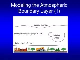
Modeling the Atmospheric Boundary Layer (2). Review of last lecture. Reynolds averaging: Separation of mean and turbulent components u = U + u’, < u’ > = 0 Intensity of turbulence: turbulent kinetic energy (TKE) Eddy fluxes Fx = - <u ’ w ’ >/z.

E N D
Review of last lecture • Reynolds averaging: Separation of mean and turbulent components u = U + u’, < u’ > = 0 • Intensity of turbulence: turbulent kinetic energy (TKE) • Eddy fluxes Fx = - <u’w’>/z TKE = ‹ u’ 2 + v’ 2 + w’ 2 ›/2
The turbulence closure problem Governing equations for the mean turbulent flow Where
The turbulence closure problem • For large-scale atmospheric circulation, we have six fundamental equations (conservation of mass, momentum, heat and water vapor) and six unknowns (p, u, v, w, T, q). So we can solve the equations to get the unknowns. • When considering turbulent motions, we have five more unknowns (eddy fluxes of u, v, w, T, q) • We have fewer fundamental equations than unknowns when dealing with turbulent motions. The search for additional laws to match the number of equations with the number of unknowns is commonly labeled the turbulence closure problem.
The current status of the turbulent closure problem • For surface layer (surface flux): nearly solvedexcept for some extreme conditions (e.g. huricane’s boundary layer) • For mixed layer: not solved. There is a variety of approaches available: (1) Local theories (2) Non-local theories However, these have not converged towards a commonly accepted BL theory, and they often show some biases when comparing with observations.
Surface layer Eddy flux is assumed to be proportional to the vertical gradience of the mean state variable • Sensible heat flux <w’h’> = Qh = Cd Cp V (Tsurface - Tair) • Latent heat flux L <w’q’> = Qe = Cd L V (qsurface - qair) Where is the air density, Cd is flux transfer coefficient, Cp is specific heat of air, V is surface wind speed, Tsurface is surface temperature, Tair is air temperature, qsurface is surface specific humidity, qair is surface air specific humidity
Mixed layer theory I: Local theories • K-theory: In eddy-diffusivity (often called K-theory) models, the turbulent flux of an adiabatically conserved quantity a (such as θ in the absence of saturation, but not temperature T, which decreases when an air parcel is adiabatically lifted) is related to its gradient: < w’a’ > = - Ka dA/dz • The local effect is always down-gradient (i.e. from high value to low value) • The key question is how to specify Ka in terms of known quantities. Three commonly used approaches: (1) First-order closure (2) 1.5-order closure or TKE closure (3) K-profile
First-order closure z Turbulent transport x z Turbulent transport x Z (by Prof. Ping Zhu of FIU)
Example: The Ekman layer • Assumption Km = constant (First order closure) • Then the boundary layer momentum equations are: • Vertical boundary conditions: • Solutions:
Ocean surface currents – horizontal water motions Transfer energy and influence overlying atmosphere Surface currents result from frictional drag caused by wind - Ekman Spiral General circulation of the oceans • Water moves at a 45o angle (right) • in N.H. to prevailing wind direction • Greater angle at depth
Global surface currents • Surface currents mainly driven by surface winds • North/ South Equatorial Currents pile water westward, create the Equatorial • Countercurrent • western ocean basins –warm poleward moving currents (example: Gulf Stream) • eastern basins –cold currents, directed equatorward
Pressure grad. force Centrifugal force Pressure grad. force Centrifugal force Secondary circulation Frictional force Inflow Pressure grad. force Centrifugal force Boundary layer Ekman pumping (by Prof. Ping Zhu of FIU)
Hurricane Vortex Pressure grad. force Coriolis force L Centrifugal force Converging Spin up Diverging Spin down Buoyancy X Ekman Pumping Boundary Layer It is the convective clouds that generate spin up process to overcome the spin down process induced by the Ekman pumping
To close the system, first order turbulent closure is to use first-order moments to parameterize second-order moments. Second order turbulent closure is to use second-order moments to parameterize third-order moments. Third order turbulent closure is to use third-order moments to parameterize fourth-order moments. Fourth order turbulent closure is to use fourth-order moments to parameterize fifth-order moments. ……… Why higher order closure is better than lower order closure? The advantage of higher-order turbulence closure is that parameterizations of unclosed higher-order moments, e.g., fourth-order moments, might be very crude, but the prognosed third-order moments can be precise since there are enough remaining physics in their budget equations. The second-order moment equations bring in more physics, making them even more precise, and so on down to the first-order moments.
Mixed layer theory II: Non-local theories • Any eddy diffusivity approach will not be entirely accurate if most of the turbulent fluxes are carried by organized eddies filling the entire boundary layer. • The non-local effect could be counter-gradient. • Consequently, a variety of ‘nonlocal’ schemes which explicitly model the effects of these boundary layer filling eddies in some way have been proposed. • A difficulty with this approach is that the structure of the turbulence depends on the BL stability, baroclinicity, history, moist processes, etc., and no nonlocal parameterization proposed to date has comprehensively addressed the effects of all these processes on the large-eddy structure. • Nonlocal schemes are most attractive when the vertical structure and turbulent transports in a specific type of boundary layer (i. e. neutral or convective) must be known to high accuracy.
Illustration of non-local turbulent mixing concept 1 1 2 2 3 3 4 4 1 1 2 2 3 3 4 4 (by Prof. Ping Zhu of FIU)
Summary • The turbulent closure problem: Number of unknowns > Number of equations • Surface layer: related to gradient • Mixed layer: Local theories (K-theory): < w’a’ >= - Ka dA/dz always down-gradient Non-local theories: organized eddies filling the entire BL, could be counter-gradient