Download
1 / 33
330 likes | 517 Views
Clustering short time series gene expression data. Jason Ernst, Gerard J. Nau and Ziv Bar-Joseph BIOINFORMATICS, vol. 21 2005. Outline. Introduction Identifying significant expression patterns Results. Introduction. More than 80% of all time series expression datasets are short

E N D
Clustering short time series gene expression data Jason Ernst, Gerard J. Nau and Ziv Bar-JosephBIOINFORMATICS, vol. 21 2005
Outline • Introduction • Identifying significant expression patterns • Results
Introduction • More than 80% of all time series expression datasets are short • Require multiple arrays making them very expensive • It is prohibitive to obtain large quantifies of biological material. Stanford Microarray Database (SMC)
Introduction • Hierarchical clustering along with other standard clustering methods • data at each time point is collected independent of each other. • Clustering using the continuous representation of the profile and clustering using a hidden Markov model • Work well for relatively long time series dataset • Not appropriate for shorter time series • Cause overfit when the number of time points is small • Most clustering algorithms cannot distinguish between patterns that occur because of random chance and clusters that represent a real response to the biological experiment.
Introduction • We present an algorithm specifically designed for clustering short time series expression data: • By assigning genes to a predefined set of model profile • How to obtain such a set of profiles • How to determine the significance of each of these profiles • Significant profiles can either be analyzed independently or they can be grouped into larger clusters.
Selecting model profiles • Selecting a set of model expression profiles • All are distinct from one another • Representative of any expression profile • Convert raw expression values into log ratios where the ratios are with respect to the expression of the first time point.
Selecting model profiles • the amount of change c a gene can exhibit between successive time points. • For example, if c=2 then between successive time points a gene can go up either one or two units, stay the same, or go down one or two units. • For n time points, this strategy results in (2c+1)n-1 distinct profiles. • Our method relies on correlation, ‘one unit’ may be defined differently for different genes.
Selecting model profiles • Selecting a (manageable) subset of the profiles • The number of profile grows as a high order polynomial in c. • For example, for 6 time points and c=2 this method results in 55=3125 models. • Too much for user to view and also likely to be very sparsely populated. • m distinct, but representative profiles.
Selecting model profiles • Computational speaking : • Let P represent the (2c+1)n-1 set of possible profiles • Select a set with m profiles • Such that the minimum distance between any two profiles in R is maximized. Where d is a distance metric.
Selecting model profiles • b(R) is the minimal distance between profiles in R • Finding the optimal value b(R’) is NP-Hard • Our greedy algorithm finds a set of profile R ,with b(R)≥ b(R’)/2 • Let R be the set of profiles selected so far. The next profile added to R is the profile p that maximized the following equation:
Selecting model profiles Greedy approximation algorithm to choose a set of m distinct profiles
Selecting model profiles • a related problem known as the k-centers problem : • Looking for a subset of R of size k such that the maximum distance from points not in R to points in R is minimized. • The k-center problem tries to select centers that are the best representatives for the group while our goal is to find the most distinct profiles.
Selecting model profiles • In general, an optimal solution to one of these problems is not necessarily an optimal solution to the other. • The algorithm we presented above is also known to be the best possible approximation algorithm for k-centers. • A distinct subset which is also a good representation of the initial set of profiles P.
Identifying significant model profiles • Given a set M of model profiles and a set of genes G, each gene is assigned to a model expression profile such that is the minimum over all . • If the above distance is minimized by h>1 model profiles then we assign g to all of these profiles, but weight the assignment in the counts as 1/h. • t(mi) : the number of gene assigned to the mi model profile
Identifying significant model profiles • Null hypothesis : Data are memoryless • The probability of observing a value at any time point is independent of past and future values • Model profiles that represent true biological function deviate significantly from the null hypothesis since many more genes than expected by random chance are assigned to them.
Identifying significant model profiles • Use a permutation based test • Permutation is used to quantify the expected number of genes that would have been assigned to each model profile if the data were generated at random. • n time points, each gene has n! possible permutations • Let be the number of genes assigned to model profile i in permutation j. • , the expected number of genes • Different model profiles may have different number of expected genes and so in general
Identifying significant model profiles • The number of genes in each profile is distributed as binomial random variable with parameters |G| and Ei/|G| • The (uncorrected) P-value of seeing t(mi) genes assigned to profile pi is , where
Identifying significant model profiles • Testing just one model expression profile: • statistically significant at the significant level if • Testing m model profile: • Apply a Bonferroni correction • Statistically significant if P(X≥t(mi)) < /m
Correlation coefficient • Correlation coefficient : (x,y) • Group together genes with similar expression profiles even if their units of change are different. • Does not satisfy the triangle inequality and thus is not a metric. • Instead we use the value gm(x,y)=1-(x,y) • Greater or equal to 0 • Satisfy a generalized version of the triangle inequality
Grouping significant profiles • We transform this problem into a graph theoretic problem • A graph (V,E), V is the set of significant model profiles • Two profiles are connected with an edge iff . • Cliques in this graph correspond to sets of significant profiles which are all similar to one another • Identifying large cliques of profiles which are all very similar to each other.
Grouping significant profiles • Greedy algorithm to partition the graph into cliques • Initially cluster Ci={pi} • Next, look for a profile pj such that pj is the closet profile to pi that is not already included in Ci . • If d(pj ,pi )≤ for all profiles pk we add pj to Ci and repeat this process, otherwise we stop and declare Ci as the cluster for pi. • After obtaining clusters for all significant profiles, we select the cluster with the largest number of genes, remove all profiles in that cluster and repeat the above process. • The algorithm terminates when all profiles have been assigned to cluster
Results • First simulated experiment • 5000 genes with 5 time points • The raw expression value at each time point was randomly draw from a uniform (10, 100) distribution. • The distribution was identical for all time points • 50 model profiles with a maximum unit change beween time points of two
Results • The region above the diagonal line corresponds to gene assignments levels that would be statistically significant. • If we assume that the number of expected genes for each profile is the same (5000/50=100) then anything above the horizontal line would be considered statistically significant.
Results • Second simulated experiment • Select three profiles and assign 50 genes (1%) to each of these profiles
Results • Biological results • Test on immune response data from Guillemin et al. • Data obtained from two replicates on the same biological sample in which time series data were collected at 5 time points, 0, 0.5, 3, 6, and 12h. • First selected 2243 genes for further analysis from the 24,192 array probes. • Genes were selected based on the agreement between the two repeats and their change at any of the experiment time points.
Results • A set of 50 model profiles • c=2 • 10 profiles in seven cluster were identified as significant
Results • Correlation of 0.7 (=0.3) • Four of the 10 significant model profiles were significantly enriched for GO categories, two of these profiles were assigned to the cluster containing three profiles
Results • Profile 9 (0,-1,-2,-3,-4) • Contain 131 genes • This profile was significantly enriched for cell-cycle genes (P-value < 10-10) • Many of the cycling genes in this profile are known transcription factors, which could contribute to repression of cell-cycles genes and ultimately the cell cycle
Results • Profile 14 (0,-1,0,3,3) • contain 49 genes • went slightly down at the beginning, but later were expressed at high levels • GO analysis indicates that many of these genes were relevant to cell structure and
Results • Profile 41 (0,1,2,3,4) • Contained 86 genes • The most enriched GO category for this profile was response to stimulus (P-value=2x10⁻⁵)