Download
1 / 54
540 likes | 701 Views
Clustering of Time Course Gene-Expression Data via Mixture Regression Models. Geoff McLachlan (joint with Angus Ng and Sam Wang) Department of Mathematics & Institute for Molecular Bioscience University of Queensland. ARC Centre of Excellence in Bioinformatics

E N D
Clustering of Time Course Gene-Expression Data via Mixture Regression Models Geoff McLachlan (joint with Angus Ng and Sam Wang) Department of Mathematics & Institute for Molecular Bioscience University of Queensland ARC Centre of Excellence in Bioinformatics http://www.maths.uq.edu.au/~gjm
Institute for Molecular Bioscience, University of Queensland
Time-Course Data Time-course microarray experiments are being increasingly used to characterize dynamic biological processes. (Microarray technology provides the ability to measure the expression levels of thousands of genes at once.) In these experiments, gene-expression levels are measured at different time points, possibly in different biological conditions (e.g. treatment-control). The focus here is on the analysis of gene-expression profiles consisting of short time series of log expression ratios for each of the genes represented on the microarrays.
CLUSTERING OF GENE PROFILES can provide new insight into the biological proces of interest (coexpressed genes can contribute to our understanding of the regulatory network of gene expression). can also assist in assigning functions to genes that have not yet been functionally annotated. a secondary concern is the need for imputation of missing data
The biological rationale underlying the clustering of microarray data is the fact that many coexpressed genes are coregulated. It becomes a way of identifying sets of genes that are putatively coregulated, thereby generating testable hypotheses; see Boutros and Okey (2005). It assists with: the functional annotation of uncharacterised genes the identification of transcription factor binding sites the elucidation of complete biological pathways
Outline of Talk • 1. Mixture model-based approach to analysis of gene-expressions • 2. Normal Mixtures • 3. Modifications for high-dimensional and/or structured data • Mixtures of linear mixed models • Clustering of gene profiles
Finite Mixture Models • Provide an arbitrarily accurate estimate of the underlying density with g sufficiently large • Provide a probabilistic clustering of the data into g clusters - outright clustering by assigning a data point to the component to which it has the greatest posterior probability of belonging.
Definition We letY1,…. Yndenote a random sample of sizenwhereYjis a p-dimensional random vector with probability density functionf (yj) where thef i(yj) are densities and thepiare nonnegative quantities that sum to one.
By Bayes Theorem, fori=1,…, g; j=1,…,n. The quantityti(yj;Y (k)) is the posterior probability that thejthmember of the sample with observed valueyjbelongs to theithcomponent of the mixture.
A soft (probabilistic) clustering is given in terms of the estimated posterior probabilities of component membership A hard (outright) clustering is given by assigning each yj to the component to which it has the highest posterior probability of belonging; that is, given by the where
Multivariate Mixture Models Day (Biometrika, 1969) Wolfe (NORMIX, 1965, 1967, 1970) It was the publication of the seminal paper ofDempster, Laird, and Rubin (1977) on theEM algorithm that greatly stimulated interest inthe use of finite mixture distributions to model heterogeneous data.
Multivariate Mixture Models Day (Biometrika, 1969) Wolfe (NORMIX, 1965, 1967, 1970) It was the publication of the seminal paper ofDempster, Laird, and Rubin (1977) on theEM algorithm that greatly stimulated interest inthe use of finite mixture distributions to model heterogeneous data. Ganesalingam and McLachlan (Biometrika,1978)
Everitt and Hand (2001) • Titterington, Smith, and Makov (1985)
Everitt and Hand (2001) • Titterington, Smith, and Makov (1985) • McLachlan and Basford (1988) • Lindsay (1996) • McLachlan and Peel (2000) • Bohning (2000) • Fruhwirth-Schnatter (2006)
Normal Mixtures Suppose that the density of the random vectorYjhas ag-component normal mixture form whereYis the vector containing the unknown parameters.
One attractive feature of adopting mixture models with elliptically symmetric components, such as the normal or t densities, is that the implied clustering is invariant under affine transformations of the data, i.e., under operations relating to changes in location, scale, and rotation of the data. Thus the clustering process does not depend on irrelevant factors such as the units of measurement or the orientation of the clusters in space.
Microarray Data represented as N x M Matrix Sample 1 Sample 2 Sample M Gene 1 Gene 2 Gene N Expression Signature M columns (samples) ~ 102 N rows (genes) ~ 104 Expression Profile
Clustering of Microarray Data Clustering of tissues on basis of genes: latter is a nonstandard problem in cluster analysis (n =M << p=N) Clustering of genes on basis of tissues: genes (observations) not independent and structure on the tissues (variables) (n=N >> p=M)
The component-covariance matrixΣiis highly parameterized withp(p+1)/2parameters. Σi= σ2Ip (equal spherical) Σi= σi2Ip(unequal spherical) Σi= D (equal diagonal) Σi= Di (unequal diagonal) Σi= Σ (equal)
Banfield and Raftery (1993) introduced a parameterization of the component-covariance matrix Σibased on a variant of the standard spectral decomposition of Σi(i=1, …,g).
However, if p is large relative to the sample size n, it may not be possible to use this decomposition to infer an appropriate model for the component-covariance matrices. Even if it is possible, the results may not be reliable due to potential problems with near-singular estimates of the component-covariance matrices when p is large relative to n.
Hence, in fitting normal mixture models to high-dimensional data, we should first consider • some form of dimension reduction and/or • some form of regularization
Mixture Software: EMMIX EMMIX for UNIX McLachlan, Peel, Adams, and Basford http://www.maths.uq.edu.au/~gjm/emmix/emmix.html
PROVIDES A MODEL-BASED APPROACH TO CLUSTERING McLachlan, Bean, and Peel, 2002, A Mixture Model-Based Approach to the Clustering of Microarray Expression Data,Bioinformatics18, 413-422 http://www.bioinformatics.oupjournals.org/cgi/screenpdf/18/3/413.pdf
Microarray Data represented as N x M Matrix Sample 1 Sample 2 Sample M Gene 1 Gene 2 Gene N Expression Signature M columns (samples) ~ 102 N rows (genes) ~ 104 Expression Profile
In applying the normal mixture model to cluster multivariate • (continuous) data, it is assumed as in most typical cluster analyses using any other method that • there are no replications on any particular entity specifically identified as such; • (b) all the observations on the entities are independent of one another
For example, where and where
Clustering of gene expression profiles • Longitudinal (with or without replication, for example time-course) • Cross-sectional data EMMIX-WIRE EM-based MIXture analysis With Random Effects Ng, McLachlan, Wang, Ben-Tovim Jones, and Ng (2006, Bioinformatics) Supplementary information : http://www.maths.uq.edu.au/~gjm/bioinf0602_supp.pdf
In the ith component of the mixture, the profile vector yj for the jth gene follows the model
Celeux et al. (2005).Mixtures of linear mixed models for clustering gene expression profiles from repeated microarray measurements. Statistical Modelling 5 , 243-267. • Qin and Self (2006).The clustering of regression models method with applications in gene expression data.Biometrics 62, 526-533. • Booth et al. (2008).Clustering using objective functions and stochastic search. J R Statist Soc B 70, 119-139.
Yeast cell cycle data of Cho et al. (1998) n=237genes at p=17 time points categorized into 4 MIPS (Munich Information Centre for Protein Sequences)functional groups. The yeast system is useful because of our ability to control and monitor the progression of cells through the cell cycle (temperature-based synchronization with temperature-sensitive genes whose product is essential for cell-cycle progression).
High-density oligonucleotide arrays were used to quanitate mRNA transcript levels in synchronized yeast cells at regular intervals (10 min) during the cell cycle (genes with cell-cycle dependent periodicity). Samples of yeast cultures were taken at 17 time points after their cell cycle phase had been synchronized. The data were reduced to a short time series of log expression ratios for each of the yeast genes represented on the microarrays (expression ratios were calculated by dividing each intensity measurement by the average for that gene.
Example . Clustering of yeast cell cycle time-course data n = 237 genes p = 17 time points where
Estimated T followingBooth et al. (2004) 0, 10, 20,…, 160 T is the period – estimated to be 73 min.
Table 1: Values of BIC for Various Levels of the Number of Components g
The use of the cluster-specific random effects terms ci leads to a clusteringthat corresponds more closely to the underlying functional groups than without their use.
Figure 1: Clusters of gene-profiles obtained by mixture of linear mixed models with cluster-specific random effects
Figure 2: Clusters of gene-profiles obtained by mixture of linear mixed models without cluster-specific random effects
Figure 3: Clusters of gene-profiles obtained by mixtures of linear mixed models with and without cluster-specific random effects
Figure 4: Plots of gene profiles grouped according to their functional grouping
Figure 5: Plots of clustered gene profiles versus functional grouping
Figure 7: Plots of Clusters of gene-profiles: Model-based clustering versus k-means