Chapter 2 Straight line motion

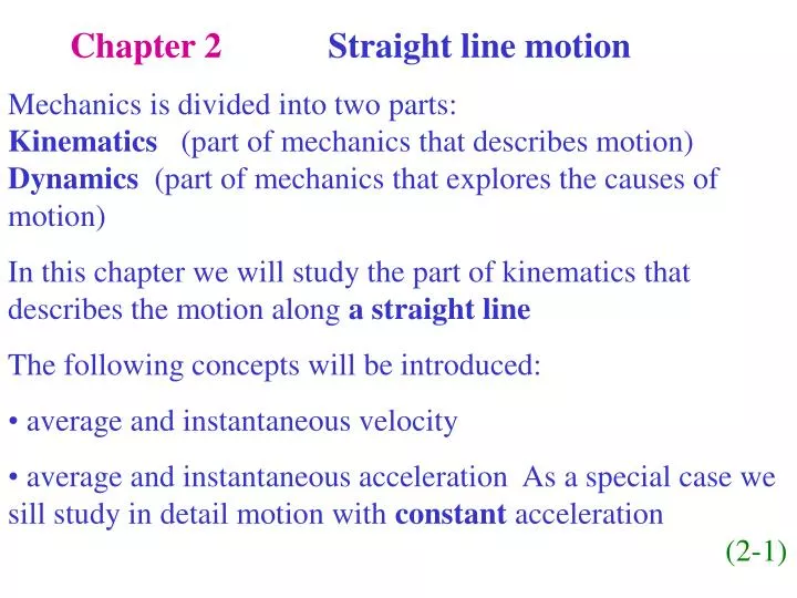
1. Chapter 2 Straight line motion • Mechanics is divided into two parts: Kinematics (part of mechanics that describes motion) Dynamics (part of mechanics that explores the causes of motion) • In this chapter we will study the part of kinematics that describes the motion along a straight line • The following concepts will be introduced: • average and instantaneous velocity • average and instantaneous acceleration As a special case we sill study in detail motion with constant acceleration (2-1)

2. Consider the motion of an athlete on a 100 m dash. How can we describe his motion? We can measure the distance x of the athlete from the start point and that time t which it takes the athlete to cover the distance x. Two such (x,t) pairs are shown in the picture at times t1 and t2 and distances x1 and x2, respectively (2,2)

3. We then plot the (x,t) pairs and get fig.a. We can pass a smooth curve through all the points and from fig.a we get fig.b. Fig.b is a plot of the distance x versus time t. Note: For motion along a straight line we do not really need to use vectors. All we have to know is whether the moving body (the athlete in this case) moves along the positive or negative direction of the x-axis . . x x axis O (2-3)

4. (2-4) Consider two snapshots of the 100 m dash athlete. At time t1 he is at distance x1 from the origin O. At a later time t2 he is at distance x2 from the origin O. We define the displacement x  x2 - x1 (units: m) Displacement describes the athlete’s change in position We define the time interval t  t2 - t1 (units: s)

5. . A Average Velocity vav units: m/s Note 1:vav is defined over the time interval from t1 to t2 Note 2:vav provides only a limited description of motion. The details of the motion are lost Extreme Example: Consider motion over a closed path. In this case x1 = x2 thus x = 0 and vav = 0 (2-5)

6. (2-6) • Determination of vav from the x versus t plot • Mark t1 and t2 on the horizontal axis • Find the corresponding positions x1 and x2 • x = x2 - x1 , t = t2 - t1 ,vav = x/ t

7. y-axis . B y2 . A y1 x-axis  O x1 x2 Mathematical note: Consider the plot of y versus x Consider points A(x1, y1) and B(x2, y2) on the curve x = x2 - x1 ,and y = y2 - y1 The limit of y/ x becomes the first derivative dy/dx of y with respect to x as x  0 Geometrically this means that B  A and that the green dotted line AB becomes the tangent at point A (red line) (2-7)

8. Instantaneous velocity v t2 = t + t x2 = x(t + t) t1= t x1= x(t) units: m/s The instantaneous velocity v is the first derivative of the function x(t) with respect to time t (2-8)

9. Example: The position of an object that moves on the x-axis is given by: x(t) = At2 + Bet + C Here,  , A, B, and C are constants Determine the instantaneous velocity v as function of t (2-9)

10. Example 2-3 (page 33) Use the graphical technique to determine v at t = 2s. We draw the tangent to the x versus t curve at t = 2 s (green line tangent at point A). We than use triangle BCD to determine the slope. D . . A C B (2-10)

11. v1 v2 Average acceleration aav units: m/s2 Instantaneous velocity v The acceleration is the first derivative of v(t) with respect to time t (2-11)

12. Example: The position of an object that moves on the x-axis is given by: x = At2 + Bet + C The velocity v was calculated on page (2-9) v = 2At + Bet Find the acceleration a as function of time t (2-12)

13. Example: Use the graphical technique to determine the acceleration a at t = 2 s a = slope at t = 2 s Draw the tangent to the v versus t curve at point A Determine the slope from triangle BCD . D A . . C B (2-13)

14. Special case: Motion with constant acceleration At t = 0 we know the initial position x(t = 0) = xo and the initial velocity v(t = 0) = vo The velocity v(t) and position x(t) at any time t are given by the following equations: If we solve eqs.1 for t we get: t = (v – vo)/a We then substitute in eqs.2 and get: eqs.1 eqs.2 eqs.3 (2-14)

15. Derivation of equation 1 a is constant  Integrate both sides with respect to time from 0 to t

16. If we plot velocity v as function of time t we get the following: v = vo + at slope = a intercept = vo The equation has the form: y = b + mx This represents a straight line with slope = m and y –axis intercept = b (2-16)

17. x x (2-17)

18. Galileo Galilei (1564-1642) He studied the laws of accelerated motion

19. Uniformly accelerated motion (a > 0) along a straight line v . a . O (2-18) x-axis Driver sees that the traffic light is green and steps on the gas v = vo + at eqs.1 x = xo + vot + at2/2 eqs 2 2a(x – xo) = v2 – vo2 eqs 3 Vector a points along the x-axis. Thus a > 0

20. Uniformly decelerated motion (a < 0) along a straight line v . a . O (2-19) x-axis Driver sees that the traffic light is red and steps on the brakes v = vo - at eqs.1 x = xo + vot - at2/2 eqs 2 -2a(x – xo) = v2 – vo2 eqs.3 Vector a points in the opposite direction of the x-axis. Thus a < 0

21. apple g . C earth g Free falling objects Close to the surface of the earth all objects move with acceleration whose magnitude g is constant g = 9.8 m/s2 Note: The vector g points towards the center of the earth (2-20)

22. Whether free fall is described by the equations of accelerated or decelerated motion depends on the choice of axes vo y vo g g O O y (2-21) g is opposite to y-axis g is parallel to y-axis Motion is decelerated Motion is accelerated v = vo – gt v = -vo + gt y = vot - gt2/2 y = -vot + gt2/2