Download
1 / 236
2.39k likes | 2.5k Views
CS4 Parallel Architectures - Introduction. Instructor : Marcelo Cintra (mc@staffmail.ed.ac.uk – 1.03 IF) Lectures: Tue and Fri in G0.9 WRB at 10am Pre-requisites: CS3 Computer Architecture Practicals: Practical 1 – out week 3 (26/1/10); due week 5 (09/2/10)

E N D
CS4 Parallel Architectures - Introduction • Instructor : Marcelo Cintra (mc@staffmail.ed.ac.uk – 1.03 IF) • Lectures: Tue and Fri in G0.9 WRB at 10am • Pre-requisites: CS3 Computer Architecture • Practicals: Practical 1 – out week 3 (26/1/10); due week 5 (09/2/10) Practical 2 – out week 5 (09/2/10); due week 7 (23/2/10) Practical 3 – out week 7 (23/2/10); due week 9 (09/3/10) (MSc only) Practical 4 – out week 7 (26/2/10); due week 9 (12/3/10) • Books: • (**) Culler & Singh - Parallel Computer Architecture: A Hardware/Software Approach – Morgan Kaufmann • (*) Hennessy & Patterson - Computer Architecture: A Quantitative Approach – Morgan Kaufmann – 3rd or 4th editions • Lecture slides (no lecture notes) • More info: www.inf.ed.ac.uk/teaching/courses/pa/ CS4/MSc Parallel Architectures - 2009-2010 1
Topics • Fundamental concepts • Performance issues • Parallelism in software • Uniprocessor parallelism • Pipelining, superscalar, and VLIW processors • Vector, SIMD processors • Interconnection networks • Routing, static and dynamic networks • Combining networks • Multiprocessors, Multicomputers, and Multithreading • Shared memory and message passing systems • Cache coherence and memory consistency • Performance and scalability CS4/MSc Parallel Architectures - 2009-2010 2
Lect. 1: Performance Issues • Why parallel architectures? • Performance of sequential architecture is limited (by technology and ultimately by the laws of physics) • Relentless increase in computing resources (transistors for logic and memory) that can no longer be exploited for sequential processing • At any point in time many important applications cannot be solved with the best existing sequential architecture • Uses of parallel architectures • To solve a single problem faster (e.g., simulating protein folding: researchweb.watson.ibm.com/bleugene) • To solve a larger version of a problem (e.g., weather forecast: www.jamstec.go.jp/esc) • To solve many problems at the same time (e.g., transaction processing) CS4/MSc Parallel Architectures - 2009-2010 3
Limits to Sequential Execution • Speed of light limit • Computation/data flow through logic gates, memory devices, and wires • At all of these there is a non-zero delay that is at a minimum equal to delay of the speed of light • Thus, the speed of light and the minimum physical feature sizes impose a hard limit on the speed of any sequential computation • Von Neumann’s limit • Programs consist of ordered sequence of instructions • Instructions are stored in memory and must be fetched in order (same for data) • Thus, sequential computation is ultimately limited by the memory bandwidth CS4/MSc Parallel Architectures - 2009-2010 4
Examples of Parallel Architectures • An ARM processor in a common mobile phone has 10s of instructions in-flight in its pipeline • Pentium IV executes up to 6 microinstructions per cycle and has up to 126 microinstructions in-flight • Intel’s quad-core chips have four processors and are now in mainstream desktops and laptops • Japan’s Earth Simulator has 5120 vector processors, each with 8 vector pipelines • IBM’s largest BlueGene supercomputer has 131,072 processors • Google has about 100,000 Linux machines connected in several cluster farms CS4/MSc Parallel Architectures - 2009-2010 5
Comparing Execution Times • Example: system A: TA execution time of program P on A system B: TB execution time of program P’ on B • Notes: • For fairness P and P’ must be “best possible implementation” on each system • If multiple programs are run then report weighted arithmetic mean • Must report all details such as: input set, compiler flags, command line arguments, etc TB Speedup: S = ; we say: A is S times faster or A is TA ( ) TB X 100 - 100 % faster TA CS4/MSc Parallel Architectures - 2009-2010 6
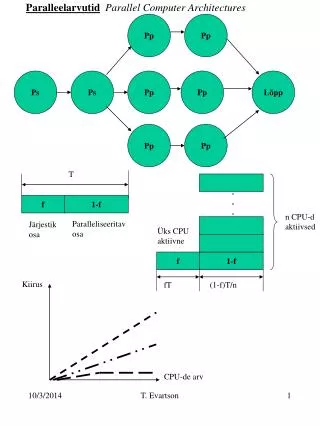
Amdahl’s Law • Let: F fraction of problem that can be optimized Sopt speedup obtained on optimized fraction • e.g.: F = 0.5 (50%), Sopt = 10 Sopt = ∞ • Bottom-line: performance improvements must be balanced 1 Soverall = F (1 – F) + Sopt 1 1 Soverall = = 1.8 Soverall = = 2 0.5 (1 – 0.5) + (1 – 0.5) + 0 10 CS4/MSc Parallel Architectures - 2009-2010 7
Amdahl’s Law and Efficiency • Let: F fraction of problem that can be parallelized Spar speedup obtained on parallelized fraction P number of processors • e.g.: 16 processors (Spar = 16), F = 0.9 (90%), • Bottom-line: for good scalability E>50%; when resources are “free” then lower efficiencies are acceptable 1 Soverall Soverall = E = F P (1 – F) + Spar 6.4 1 Soverall = = 6.4 E = = 0.4 (40%) 0.9 16 (1 – 0.9) + 16 CS4/MSc Parallel Architectures - 2009-2010 8
Performance Trends: Computer Families • Bottom-line: microprocessors have become the building blocks of most computer systems across the whole range of price-performance Culler and Singh Fig. 1.1 CS4/MSc Parallel Architectures - 2009-2010 9
Technological Trends: Moore’s Law • Bottom-line: overwhelming number of transistors allow for incredibly complex and highly integrated systems CS4/MSc Parallel Architectures - 2009-2010 10
Tracking Technology: The role of CA • Bottom-line: architectural innovation complement technological improvements H&P Fig. 1.1 CS4/MSc Parallel Architectures - 2009-2010 11
The Memory Gap • Bottom-line: memory access is increasingly expensive and CA must devise new ways of hiding this cost H&P Fig. 5.2 CS4/MSc Parallel Architectures - 2009-2010 12
Software Trends • Ever larger applications: memory requirements double every year • More powerful compilers and increasing role of compilers on performance • Novel applications with different demands: e.g., multimedia • Streaming data • Simple fixed operations on regular and small data MMX-like instructions e.g., web-based services • Huge data sets with little locality of access • Simple data lookups and processing Transactional Memory(?) (www.cs.wisc.edu/trans-memory) • Bottom-line: architecture/compiler co-design CS4/MSc Parallel Architectures - 2009-2010 13
Current Trends in CA • Very complex processor design: • Hybrid branch prediction (MIPS R14000) • Out-of-order execution (Pentium IV) • Multi-banked on-chip caches (Alpha 21364) • EPIC (Explicitly Parallel Instruction Computer) (Intel Itanium) • Parallelism and integration at chip level: • Chip-multiprocessors (CMP) (Sun T2, IBM Power6, Intel Itanium 2) • Multithreading (Intel Hyperthreading, IBM Power6, Sun T2) • Embedded Systems On a Chip (SOC) • Multiprocessors: • Servers (Sun Fire, SGI Origin) • Supercomputers (IBM BlueGene, SGI Origin, IBM HPCx) • Clusters of workstations (Google server farm) • Power-conscious designs CS4/MSc Parallel Architectures - 2009-2010 14
Lect. 2: Types of Parallelism • Parallelism in Hardware (Uniprocessor) • Parallel arithmetic • Pipelining • Superscalar, VLIW, SIMD, and vector execution • Parallelism in Hardware (Multiprocessor) • Chip-multiprocessors a.k.a. Multi-cores • Shared-memory multiprocessors • Distributed-memory multiprocessors • Multicomputers a.k.a. clusters • Parallelism in Software • Tasks • Data parallelism • Data streams (note: a “processor” must be capable of independent control and of operating on non-trivial data types) CS4/MSc Parallel Architectures - 2009-2010 1
Taxonomy of Parallel Computers • According to instruction and data streams (Flynn): • Single instruction single data (SISD): this is the standard uniprocessor • Single instruction, multiple data streams (SIMD): • Same instruction is executed in all processors with different data • E.g., graphics processing • Multiple instruction, single data streams (MISD): • Different instructions on the same data • Never used in practice • Multiple instruction, multiple data streams (MIMD): the “common” multiprocessor • Each processor uses it own data and executes its own program (or part of the program) • Most flexible approach • Easier/cheaper to build by putting together “off-the-shelf” processors CS4/MSc Parallel Architectures - 2009-2010 2
Taxonomy of Parallel Computers • According to physical organization of processors and memory: • Physically centralized memory, uniform memory access (UMA) • All memory is allocated at same distance from all processors • Also called symmetric multiprocessors (SMP) • Memory bandwidth is fixed and must accommodate all processors does not scale to large number of processors • Used in most CMPs today (e.g., IBM Power5, Intel Core Duo) CPU CPU CPU CPU Cache Cache Cache Cache Interconnection Main memory CS4/MSc Parallel Architectures - 2009-2010 3
Taxonomy of Parallel Computers • According to physical organization of processors and memory: • Physically distributed memory, non-uniform memory access (NUMA) • A portion of memory is allocated with each processor (node) • Accessing local memory is much faster than remote memory • If most accesses are to local memory than overall memory bandwidth increases linearly with the number of processors CPU CPU CPU CPU Node Cache Cache Cache Cache Mem. Mem. Mem. Mem. Interconnection CS4/MSc Parallel Architectures - 2009-2010 4
Taxonomy of Parallel Computers • According to memory communication model • Shared address or shared memory • Processes in different processors can use the same virtual address space • Any processor can directly access memory in another processor node • Communication is done through shared memory variables • Explicit synchronization with locks and critical sections • Arguably easier to program • Distributed address or message passing • Processes in different processors use different virtual address spaces • Each processor can only directly access memory in its own node • Communication is done through explicit messages • Synchronization is implicit in the messages • Arguably harder to program • Some standard message passing libraries (e.g., MPI) CS4/MSc Parallel Architectures - 2009-2010 5
Shared Memory vs. Message Passing • Shared memory • Message passing Producer (p1) Consumer (p2) flag = 0; … a = 10; flag = 1; flag = 0; … while (!flag) {} x = a * y; Producer (p1) Consumer (p2) … a = 10; send(p2, a, label); … receive(p1, b, label); x = b * y; CS4/MSc Parallel Architectures - 2009-2010 6
Types of Parallelism in Applications • Instruction-level parallelism (ILP) • Multiple instructions from the same instruction stream can be executed concurrently • Generated and managed by hardware (superscalar) or by compiler (VLIW) • Limited in practice by data and control dependences • Thread-level or task-level parallelism (TLP) • Multiple threads or instruction sequences from the same application can be executed concurrently • Generated by compiler/user and managed by compiler and hardware • Limited in practice by communication/synchronization overheads and by algorithm characteristics CS4/MSc Parallel Architectures - 2009-2010 7
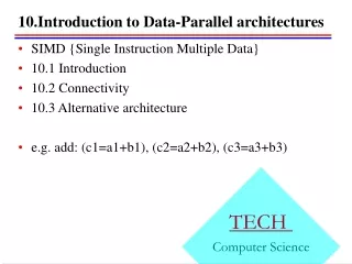
Types of Parallelism in Applications • Data-level parallelism (DLP) • Instructions from a single stream operate concurrently (temporally or spatially) on several data • Limited by non-regular data manipulation patterns and by memory bandwidth • Transaction-level parallelism • Multiple threads/processes from different transactions can be executed concurrently • Sometimes not really considered as parallelism • Limited by access to metadata and by interconnection bandwidth CS4/MSc Parallel Architectures - 2009-2010 8
Example: Equation Solver Kernel • The problem: • Operate on a (n+2)x(n+2) matrix • Points on the rim have fixed value • Inner points are updated as: • Updates are in-place, so top and left are new values and bottom and right are old ones • Updates occur at multiple sweeps • Keep difference between old and new values and stop when difference for all points is small enough A[i,j] = 0.2 x (A[i,j] + A[i,j-1] + A[i-1,j] + A[i,j+1] + A[i+1,j]) CS4/MSc Parallel Architectures - 2009-2010 9
Example: Equation Solver Kernel • Dependences: • Computing the new value of a given point requires the new value of the point directly above and to the left • By transitivity, it requires all points in the sub-matrix in the upper-left corner • Points along the top-right to bottom-left diagonals can be computed independently CS4/MSc Parallel Architectures - 2009-2010 10
Example: Equation Solver Kernel • ILP version (from sequential code): • Machine instructions from each j iteration can occur in parallel • Branch prediction allows overlap of multiple iterations of j loop • Some of the instructions from multiple j iterations can occur in parallel while (!done) { diff = 0; for (i=1; i<=n; i++) { for (j=1; j<=n; j++) { temp = A[i,j]; A[i,j] = 0.2*(A[i,j]+A[i,j-1]+A[i-1,j] + A[i,j+1]+A[i+1,j]); diff += abs(A[i,j] – temp); } } if (diff/(n*n) < TOL) done=1; } CS4/MSc Parallel Architectures - 2009-2010 11
Example: Equation Solver Kernel • TLP version (shared-memory): int mymin = 1+(pid * n/P); int mymax = mymin + n/P – 1; while (!done) { diff = 0; mydiff = 0; for (i=mymin; i<=mymax; i++) { for (j=1; j<=n; j++) { temp = A[i,j]; A[i,j] = 0.2*(A[i,j]+A[i,j-1]+A[i-1,j] + A[i,j+1]+A[i+1,j]); mydiff += abs(A[i,j] – temp); } } lock(diff_lock); diff += mydiff; unlock(diff_lock); barrier(bar, P); if (diff/(n*n) < TOL) done=1; barrier(bar, P); } CS4/MSc Parallel Architectures - 2009-2010 12
Example: Equation Solver Kernel • TLP version (shared-memory) (for 2 processors): • Each processor gets a chunk of rows • E.g., processor 0 gets: mymin=1 and mymax=2 and processor 1 gets: mymin=3 and mymax=4 int mymin = 1+(pid * n/P); int mymax = mymin + n/P – 1; while (!done) { diff = 0; mydiff = 0; for (i=mymin; i<=mymax; i++) { for (j=1; j<=n; j++) { temp = A[i,j]; A[i,j] = 0.2*(A[i,j]+A[i,j-1]+A[i-1,j] + A[i,j+1]+A[i+1,j]); mydiff += abs(A[i,j] – temp); } ... CS4/MSc Parallel Architectures - 2009-2010 13
Example: Equation Solver Kernel • TLP version (shared-memory): • All processors can access freely the same data structure A • Access to diff, however, must be in turns • All processors update together their own done variable ... for (i=mymin; i<=mymax; i++) { for (j=1; j<=n; j++) { temp = A[i,j]; A[i,j] = 0.2*(A[i,j]+A[i,j-1]+A[i-1,j] + A[i,j+1]+A[i+1,j]); mydiff += abs(A[i,j] – temp); } } lock(diff_lock); diff += mydiff; unlock(diff_lock); barrier(bar, P); if (diff/(n*n) < TOL) done=1; barrier(bar, P); } CS4/MSc Parallel Architectures - 2009-2010 14
Types of Speedups and Scaling • Scalability: adding x times more resources to the machine yields close to x times better “performance” • Usually resources are processors, but can also be memory size or interconnect bandwidth • Usually means that with x times more processors we can get ~x times speedup for the same problem • In other words: How does efficiency (see Lecture 1) hold as the number of processors increases? • In reality we have different scalability models: • Problem constrained • Time constrained • Memory constrained • Most appropriate scalability model depends on the user interests CS4/MSc Parallel Architectures - 2009-2010 15
Types of Speedups and Scaling • Problem constrained (PC) scaling: • Problem size is kept fixed • Wall-clock execution time reduction is the goal • Number of processors and memory size are increased • “Speedup” is then defined as: • Example: CAD tools that take days to run, weather simulation that does not complete in reasonable time Time(1 processor) SPC = Time(p processors) CS4/MSc Parallel Architectures - 2009-2010 16
Types of Speedups and Scaling • Time constrained (TC) scaling: • Maximum allowable execution time is kept fixed • Problem size increase is the goal • Number of processors and memory size are increased • “Speedup” is then defined as: • Example: weather simulation with refined grid Work(p processors) STC = Work(1 processor) CS4/MSc Parallel Architectures - 2009-2010 17
Types of Speedups and Scaling • Memory constrained (MC) scaling: • Both problem size and execution time are allowed to increase • Problem size increase with the available memory with smallest increase in execution time is the goal • Number of processors and memory size are increased • “Speedup” is then defined as: • Example: astrophysics simulation with more planets and stars Work(p processors) Time(1 processor) Increase in Work SMC = x = Time(p processors) Work(1 processor) Increase in Time CS4/MSc Parallel Architectures - 2009-2010 18
Lect. 3: Superscalar Processors I/II • Pipelining: several instructions are simultaneously at different stages of their execution • Superscalar: several instructions are simultaneously at the same stages of their execution • (Superpipelining: very deep pipeline with very short stages to increase the amount of parallelism) • Out-of-order execution: instructions can be executed in an order different from that specified in the program • Dependences between instructions: • Read after Write (RAW) (a.k.a. data dependence) • Write after Read (WAR) (a.k.a. anti dependence) • Write after Write (WAW) (a.k.a. output dependence) • Control dependence • Speculative execution: tentative execution despite dependences CS4/MSc Parallel Architectures - 2009-2010 1
A 5-stage Pipeline Memory Memory General registers IF ID EXE MEM WB IF = instruction fetch (includes PC increment) ID = instruction decode + fetching values from general purpose registers EXE = arithmetic/logic operations or address computation MEM = memory access or branch completion WB = write back results to general purpose registers CS4/MSc Parallel Architectures - 2009-2010 2
A Pipelining Diagram • Start one instruction per clock cycle IF I1 I2 I3 I4 I5 I6 instruction flow I1 I2 I3 I4 I5 ID I1 I2 I3 I4 EXE I1 I2 I3 MEM I1 I2 WB cycle 1 2 3 4 5 6 each instruction still takes 5 cycles, but instructions now complete every cycle: CPI 1 CS4/MSc Parallel Architectures - 2009-2010 3
Multiple-issue • Start two instructions per clock cycle IF I1 I3 I5 I7 I9 I11 instruction flow I2 I4 I6 I8 I10 I12 I1 I3 I5 I7 I9 ID I2 I4 I6 I8 I10 I1 I3 I5 I7 EXE CPI 0.5; IPC 2 I2 I4 I6 I8 I1 I3 I5 MEM I2 I4 I6 I1 I3 WB I2 I4 cycle 1 2 3 4 5 6 CS4/MSc Parallel Architectures - 2009-2010 4
A Pipelined Processor (DLX) H&P Fig. A.18 CS4/MSc Parallel Architectures - 2009-2010 5
Advanced Superscalar Execution • Ideally: in an n-issue superscalar, n instructions are fetched, decoded, executed, and committed per cycle • In practice: • Control flow changes spoil fetch flow • Data, control, and structural hazards spoil issue flow • Multi-cycle arithmetic operations spoil execute flow • Buffers at issue (issue window or issue queue) and commit (reorder buffer) decouple these stages from the rest of the pipeline and regularize somewhat breaks in the flow Memory Memory General registers instructions instructions Fetch engine ID EXE MEM WB CS4/MSc Parallel Architectures - 2009-2010 6
Problems At Instruction Fetch • Crossing instruction cache line boundaries • e.g., 32 bit instructions and 32 byte instruction cache lines → 8 instructions per cache line; 4-wide superscalar processor • More than one cache lookup are required in the same cycle • What if one of the line accesses is a cache miss? • Words from different lines must be ordered and packed into instruction queue Case 1: all instructions located in same cache line and no branch Case 2: instructions spread in more lines and no branch CS4/MSc Parallel Architectures - 2009-2010 7
Problems At Instruction Fetch • Control flow • e.g., 32 bit instructions and 32 byte instruction cache lines → 8 instructions per cache line; 4-wide superscalar processor • Branch prediction is required within the instruction fetch stage • For wider issue processors multiple predictions are likely required • In practice most fetch units only fetch up to the first predicted taken branch Case 1: single not taken branch Case 2: single taken branch outside fetch range and into other cache line CS4/MSc Parallel Architectures - 2009-2010 8
Example Frequencies of Control Flow • One branch/jump about every 4 to 6 instructions • One taken branch/jump about every 4 to 9 instructions Data from Rotenberg et. al. for SPEC 92 Int CS4/MSc Parallel Architectures - 2009-2010 9
Solutions For Instruction Fetch • Advanced fetch engines that can perform multiple cache line lookups • E.g., interleaved I-caches where consecutive program lines are stored in different banks that can accessed in parallel • Very fast, albeit not very accurate branch predictors (e.g., next line predictor in the Alpha 21464) • Note: usually used in conjunction with more accurate but slower predictors (see Lecture 4) • Restructuring instruction storage to keep commonly consecutive instructions together (e.g., Trace cache in Pentium 4) CS4/MSc Parallel Architectures - 2009-2010 10
Control flow prediction • units: • Branch Target Buffer • Return Address Stack • Branch Predictor Mask to select instructions from each of the cache lines 2-way interleaved I-cache Final alignment unit Example Advanced Fetch Unit Figure from Rotenberg et. al. CS4/MSc Parallel Architectures - 2009-2010 11
Trace Caches • Traditional I-cache: instructions laid out in program order • Dynamic execution order does not always follow program order (e.g., taken branches) and the dynamic order also changes • Idea: • Store instructions in execution order (traces) • Traces can start with any static instruction and are identified by the starting instruction’s PC • Traces are dynamically created as instructions are normally fetched and branches are resolved • Traces also contain the outcomes of the implicitly predicted branches • When the same trace is again encountered (i.e., same starting instruction and same branch predictions) instructions are obtained from trace cache • Note that multiple traces can be stored with the same starting instruction CS4/MSc Parallel Architectures - 2009-2010 12
Pros/Cons of Trace Caches • Instructions come from a single trace cache line • Branches are implicitly predicted • The instruction that follows the branch is fixed in the trace and implies the branch’s direction (taken or not taken) • I-cache still present, so no need to change cache hierarchy • In CISC IS’s (e.g., x86) the trace cache can keep decoded instructions (e.g., Pentium 4) • Wasted storage as instructions appear in both I-cache and trace cache, and in possibly multiple trace cache lines • Not very good at handling indirect jumps and returns (which have multiple targets, instead of only taken/not taken) and even unconditional branches • Not very good when there are traces with common sub-paths CS4/MSc Parallel Architectures - 2009-2010 13
Structure of a Trace Cache Figure from Rotenberg et. al. CS4/MSc Parallel Architectures - 2009-2010 14
Structure of a Trace Cache • Each line contains n instructions from up to m basic blocks • Control bits: • Valid • Tag • Branch flags and mask: m-1 bits to specify the direction of the up to m branches • Branch mask: the number of branches in the trace • Trace target address and fall-through address: the address of the next instruction to be fetched after the trace is exhausted • Trace cache hit: • Tag must match • Branch predictions must match the branch flags for all branches in the trace CS4/MSc Parallel Architectures - 2009-2010 15
Trace Creation • Starts on a trace cache miss • Instructions are fetched up to the first predicted taken branch • Instructions are collected, possibly from multiple basic blocks (when branches are predicted taken) • Trace is terminated when either n instructions or m branches have been added • Trace target/fall-through address are computed at the end CS4/MSc Parallel Architectures - 2009-2010 16
I1 I2 I3 I4 I5 I6 I7 I8 I9 I10 I11 I12 I13 I14 I15 I16 I17 I18 I19 Example • I-cache lines contain 8 32-bit instructions and Trace Cache lines contain up to 24 instructions and 3 branches • Processor can issue up to 4 instructions per cycle Machine Code Basic Blocks Layout in I-Cache L1: I1 [ALU] ... I5 [Cond. Br. to L3] L2: I6 [ALU] ... I12 [Jump to L4] L3: I13 [ALU] ... I18 [ALU] L4: I19 [ALU] ... I24 [Cond. Br. to L1] B1 (I1-I5) B2 (I6-I12) B3 (I13-I18) I20 I21 I22 I23 I24 B4 (I19-I24) CS4/MSc Parallel Architectures - 2009-2010 17
I1 I2 I3 I4 I5 I6 I7 I8 I9 I10 I11 I12 I13 I14 I15 I16 I17 I18 I19 I20 I21 I22 I23 I24 Example • Step 1: fetch I1-I3 (stop at end of line) → Trace Cache miss → Start trace collection • Step 2: fetch I4-I5 (possible I-cache miss) (stop at predicted taken branch) • Step 3: fetch I13-16 (possible I-cache miss) • Step 4: fetch I17-I19 (I18 is predicted not taken branch, stop at end of line) • Step 5: fetch I20-I23 (possible I-cache miss) (stop at predicted taken branch) • Step 6: fetch I24-I27 • Step 7: fetch I1-I4 replaced by Trace Cache access Basic Blocks Layout in I-Cache Layout in Trace Cache B1 (I1-I5) I1 I2 I3 I4 I5 I13 I14 I15 I16 I17 I18 I19 I20 I21 I22 I23 I24 B2 (I6-I12) B3 (I13-I18) Common path B4 (I19-I24) CS4/MSc Parallel Architectures - 2009-2010 18