Download
1 / 37
380 likes | 481 Views
Introduction to Parallel Architectures and Programming Models. A generic parallel architecture. P. P. P. P. M. M. M. M. Interconnection Network. Memory. Where is the memory physically located?. Classifying computer architecture.

E N D
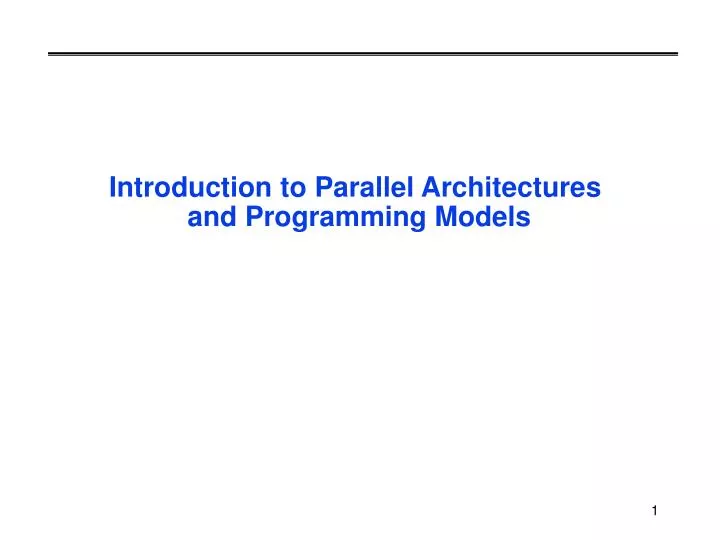
Introduction to Parallel Architectures and Programming Models
A generic parallel architecture P P P P M M M M Interconnection Network Memory • Where is the memory physically located?
Classifying computer architecture • Computer are often classified using two different measures • (Flynn’s taxonomy) • memory • shared memory • distributed memory • instruction stream and data stream Data stream single multiple single Instruction stream multiple
Parallel Programming Models • Control • How is parallelism created? • What orderings exist between operations? • How do different threads of control synchronize? • Data • What data is private vs. shared? • How is logically shared data accessed or communicated? • Operations • What are the atomic operations? • Cost • How do we account for the cost of each of the above?
Simple Example Consider a sum of an array function: • Parallel Decomposition: • Each evaluation and each partial sum is a task. • Assign n/p numbers to each of p procs • Each computes independent “private” results and partial sum. • One (or all) collects the p partial sums and computes the global sum. Two Classes of Data: • Logically Shared • The original n numbers, the global sum. • Logically Private • The individual function evaluations. • What about the individual partial sums?
i res s . . . P P P Programming Model 1: Shared Memory • Program is a collection of threads of control. • Many languages allow threads to be created dynamically, I.e., mid-execution. • Each thread has a set of private variables, e.g. local variables on the stack. • Collectively with a set of shared variables, e.g., static variables, shared common blocks, global heap. • Threads communicate implicitly by writing and reading shared variables. • Threads coordinate using synchronization operations on shared variables Address: x = ... Shared y = ..x ... Private i res s
P1 P2 Pn network memory $ $ $ Machine Model 1a: Shared Memory • Processors all connected to a large shared memory. • Typically called Symmetric Multiprocessors (SMPs) • Sun, DEC, Intel, IBM SMPs • “Local” memory is not (usually) part of the hardware. • Cost: much cheaper to access data in cache than in main memory. • Difficulty scaling to large numbers of processors • <10 processors typical
P2 $ $ $ Machine Model 1b: Distributed Shared Memory • Memory is logically shared, but physically distributed • Any processor can access any address in memory • Cache lines (or pages) are passed around machine • SGI Origin is canonical example (+ research machines) • Scales to 100s • Limitation is cache consistency protocols – need to keep cached copies of the same address consistent P1 Pn network memory memory memory
Shared Memory Code for Computing a Sum static int s = 0; Thread 1 local_s1= 0 for i = 0, n/2-1 local_s1 = local_s1 + f(A[i]) s = s + local_s1 Thread 2 local_s2 = 0 for i = n/2, n-1 local_s2= local_s2 + f(A[i]) s = s +local_s2 What is the problem? • A race condition or data race occurs when: • two processors (or two threads) access the same variable, and at least one does a write. • The accesses are concurrent (not synchronized)
Pitfalls and Solution via Synchronization • Pitfall in computing a global sum s = s + local_si: Thread 1 (initially s=0) load s [from mem to reg] s = s+local_s1 [=local_s1, in reg] store s [from reg to mem] Thread 2 (initially s=0) load s [from mem to reg; initially 0] s = s+local_s2 [=local_s2, in reg] store s [from reg to mem] Time • Instructions from different threads can be interleaved arbitrarily. • One of the additions may be lost • Possible solution: mutual exclusion with locks Thread 1 lock load s s = s+local_s1 store s unlock Thread 2 lock load s s = s+local_s2 store s unlock
send P0,X recv Pn,Y X Y i res s i res s . . . P P P Programming Model 2: Message Passing • Program consists of a collection of named processes. • Usually fixed at program startup time • Thread of control plus local address space -- NO shared data. • Logically shared data is partitioned over local processes. • Processes communicate by explicit send/receive pairs • Coordination is implicit in every communication event. • MPI is the most common example A: A: 0 n
P1 P2 Pn NI NI NI memory memory memory . . . interconnect Machine Model 2: Distributed Memory • Cray T3E, IBM SP. • Each processor is connected to its own memory and cache but cannot directly access another processor’s memory. • Each “node” has a network interface (NI) for all communication and synchronization.
Computing s = x(1)+x(2) on each processor • First possible solution: Processor 2 receive xremote, proc1 send xlocal, proc1 [xlocal = x(2)] s = xlocal + xremote Processor 1 send xlocal, proc2 [xlocal = x(1)] receive xremote, proc2 s = xlocal + xremote • Second possible solution -- what could go wrong? Processor 1 send xlocal, proc2 [xlocal = x(1)] receive xremote, proc2 s = xlocal + xremote Processor 2 send xlocal, proc1 [xlocal = x(2)] receive xremote, proc1 s = xlocal + xremote • What if send/receive acts like the telephone system? The post office?
Programming Model 2b: Global Addr Space • Program consists of a collection of named processes. • Usually fixed at program startup time • Local and shared data, as in shared memory model • But, shared data is partitioned over local processes • Remote data stays remote on distributed memory machines • Processes communicate by writes to shared variables • Explicit synchronization needed to coordinate • UPC, Titanium, Split-C are some examples • Global Address Space programming is an intermediate point between message passing and shared memory • Most common on a the Cray t3e, which had some hardware support for remote reads/writes
A: f fA: sum Programming Model 3: Data Parallel • Single thread of control consisting of parallel operations. • Parallel operations applied to all (or a defined subset) of a data structure, usually an array • Communication is implicit in parallel operators • Elegant and easy to understand and reason about • Coordination is implicit – statements executed synchronousl • Drawbacks: • Not all problems fit this model • Difficult to map onto coarse-grained machines A = array of all data fA = f(A) s = sum(fA) s:
P1 P2 Pn NI NI NI memory memory memory Machine Model 3a: SIMD System • A large number of (usually) small processors. • A single “control processor” issues each instruction. • Each processor executes the same instruction. • Some processors may be turned off on some instructions. • Machines are not popular (CM2), but programming model is. control processor . . . interconnect • Implemented by mapping n-fold parallelism to p processors. • Mostly done in the compilers (e.g., HPF).
Model 3B: Vector Machines • Vector architectures are based on a single processor • Multiple functional units • All performing the same operation • Instructions may specific large amounts of parallelism (e.g., 64-way) but hardware executes only a subset in parallel • Historically important • Overtaken by MPPs in the 90s • Still visible as a processor architecture within an SMP
Machine Model 4: Clusters of SMPs • SMPs are the fastest commodity machine, so use them as a building block for a larger machine with a network • Common names: • CLUMP = Cluster of SMPs • Hierarchical machines, constellations • Most modern machines look like this: • IBM SPs, Compaq Alpha, (not the t3e)... • What is an appropriate programming model #4 ??? • Treat machine as “flat”, always use message passing, even within SMP (simple, but ignores an important part of memory hierarchy). • Shared memory within one SMP, but message passing outside of an SMP.
Summary so far • Historically, each parallel machine was unique, along with its programming model and programming language • You had to throw away your software and start over with each new kind of machine - ugh • Now we distinguish the programming model from the underlying machine, so we can write portably correct code, that runs on many machines • MPI now the most portable option, but can be tedious • Writing portably fast code requires tuning for the architecture • Algorithm design challenge is to make this process easy • Example: picking a blocksize, not rewriting whole algorithm
Creating a Parallel Program • Pieces of the job • Identify work that can be done in parallel • Partition work and perhaps data among processes=threads • Manage the data access, communication, synchronization • Goal: maximize Speedup due to parallelism Speedupprob(P procs) = Time to solve prob with “best” sequential solution Time to solve prob in parallel on P processors <= P (Brent’s Theorem) Efficiency(P) = Speedup(P) / P <= 1
Mapping Decomposition Orchestration Assignment Overall Computation Grains of Work Processes/ Threads Processes/ Threads Processors Steps in the Process • Task: arbitrarily defined piece of work that forms the basic unit of concurrency • Process/Thread: abstract entity that performs tasks • tasks are assigned to threads via an assignment mechanism • threads must coordinate to accomplish their collective tasks • Processor: physical entity that executes a thread
Decomposition • Break the overall computation into grains of work (tasks) • identify concurrency and decide at what level to exploit it • concurrency may be statically identifiable or may vary dynamically • it may depend only on problem size, or it may depend on the particular input data • Goal: enough tasks to keep the target range of processors busy, but not too many • establishes upper limit on number of useful processors (i.e., scaling)
Assignment • Determine mechanism to divide work among threads • functional partitioning • assign logically distinct aspects of work to different threads • eg pipelining • structural mechanisms • assign iterations of “parallel loop” according to simple rule • eg proc j gets iterates j*n/p through (j+1)*n/p-1 • throw tasks in a bowl (task queue) and let threads feed • data/domain decomposition • data describing the problem has a natural decomposition • break up the data and assign work associated with regions • eg parts of physical system being simulated • Goal • Balance the workload to keep everyone busy (all the time) • Allow efficient orchestration
Orchestration • Provide a means of • naming and accessing shared data, • communication and coordination among threads of control • Goals: • correctness of parallel solution • respect the inherent dependencies within the algorithm • avoid serialization • reduce cost of communication, synchronization, and management • preserve locality of data reference
Mapping • Binding processes to physical processors • Time to reach processor across network does not depend on which processor (roughly) • lots of old literature on “network topology”, no longer so important • Basic issue is how many remote accesses Proc Proc fast Cache Cache slow really slow Memory Memory Network
Example • s = f(A[1]) + … + f(A[n]) • Decomposition • computing each f(A[j]) • n-fold parallelism, where n may be >> p • computing sum s • Assignment • thread k sums sk = f(A[k*n/p]) + … + f(A[(k+1)*n/p-1]) • thread 1 sums s = s1+ … + sp (for simplicity of this example) • thread 1 communicates s to other threads • Orchestration • starting up threads • communicating, synchronizing with thread 1 • Mapping • processor j runs thread j
Identifying enough Concurrency • Parallelism profile • area is total work done n n x time(f) Simple Decomposition: f ( A[i] ) is the parallel task sum is sequential Concurrency 1 x time(sum(n)) Time • Amdahl’s law • let s be the fraction of total work done sequentially After mapping p Concurrency p x n/p x time(f)
p x time(sum(n/p) ) Concurrency 1 x time(sum(log_2 p)) p x n/p x time(f) Algorithmic Trade-offs • Parallelize partial sum of the f’s • what fraction of the computation is “sequential” • what does this do for communication? locality? • what if you sum what you “own” • Parallelize the final summation (tree sum) • Generalize Amdahl’s law for arbitrary “ideal” parallelism profile p x time(sum(n/p) ) Concurrency 1 x time(sum(p)) p x n/p x time(f)
Problem Size is Critical Amdahl’s Law Bounds • Suppose Total work= n + P • Serial work: P • Parallel work: n • s = serial fraction • = P/ (n+P) n In general seek to exploit a fraction of the peak parallelism in the problem.
Load Balance • Insufficient Concurrency will appear as load imbalance • Use of coarser grain tends to increase load imbalance. • Poor assignment of tasks can cause load imbalance. • Synchronization waits are instantaneous load imbalance Idle Time if n does not divide by P Idle Time due to serialization Concurrency Work ( 1 ) £ Speedup ( P ) + Work ( p ) idle ) max ( p
Extra Work • There is always some amount of extra work to manage parallelism • e.g., to decide who is to do what Concurrency Work ( 1 ) £ Speedup ( P ) + + Work ( p ) idle extra ) Max ( p
Communication and Synchronization Coordinating Action (synchronization) requires communication Concurrency Getting data from where it is produced to where it is used does too. • There are many ways to reduce communication costs.
Reducing Communication Costs • Coordinating placement of work and data to eliminate unnecessary communication • Replicating data • Redundant work • Performing required communication efficiently • e.g., transfer size, contention, machine specific optimizations
The Tension Minimizing one tends to increase the others • Fine grain decomposition and flexible assignment tends to minimize load imbalance at the cost of increased communication • In many problems communication goes like the surface-to-volume ratio • Larger grain => larger transfers, fewer synchronization events • Simple static assignment reduces extra work, but may yield load imbalance
The Good News • The basic work component in the parallel program may be more efficient that in the sequential case • Only a small fraction of the problem fits in cache • Need to chop problem up into pieces and concentrate on them to get good cache performance. • Indeed, the best sequential program may emulate the parallel one. • Communication can be hidden behind computation • May lead to better algorithms for memory hierarchies • Parallel algorithms may lead to better serial ones • parallel search may explore space more effectively