Download
1 / 1
10 likes | 153 Views
A000. A1-11. A1-1-1. 1. object modeling. K x (i,j)/a*. 2. wave simulation. A-111. A-11-1. A-220. object wave amplitude. r e p e t i t i o n. FT. set 1: Ge set 2: CdTe dV o /V o = 0.02% dV’ o /V’ o = 0.8%. ?. Ge-CdTe, 300kV Sample: D. Smith

E N D
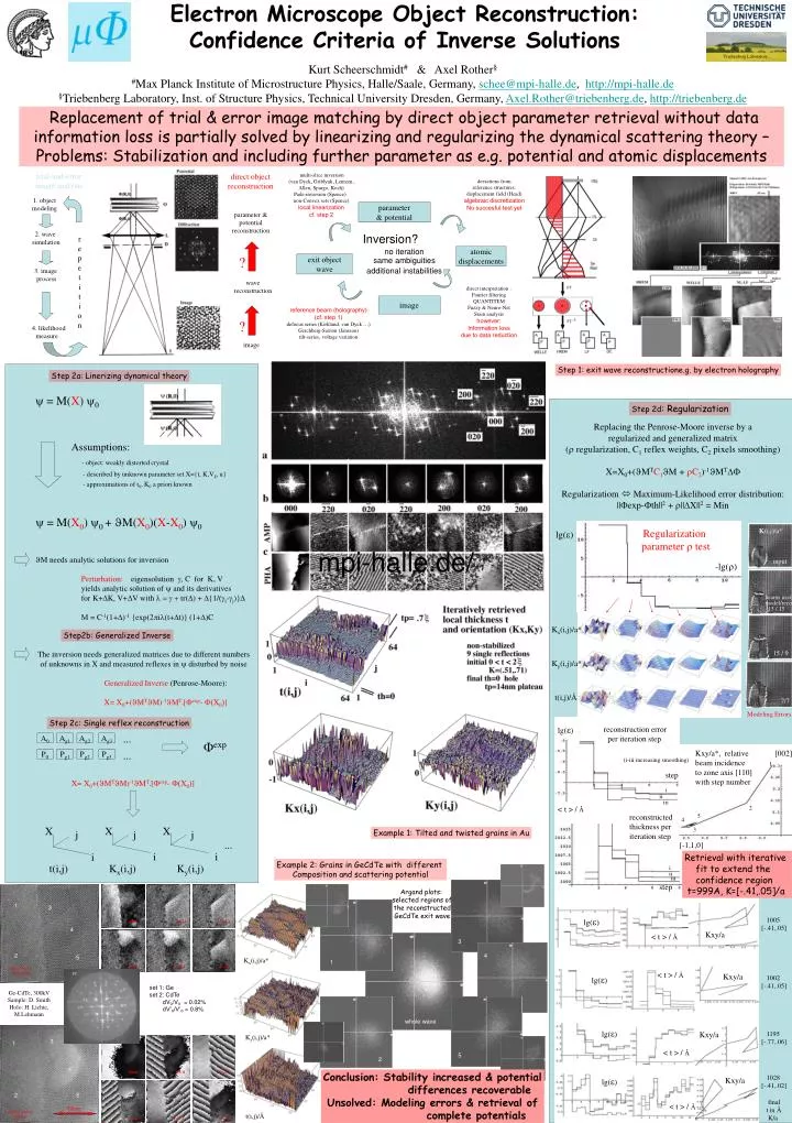
A000 A1-11 A1-1-1 1. object modeling Kx(i,j)/a* 2. wave simulation A-111 A-11-1 A-220 object wave amplitude r e p e t i t i o n FT set 1: Ge set 2: CdTe dVo/Vo = 0.02% dV’o/V’o = 0.8% ? Ge-CdTe, 300kV Sample: D. Smith Holo: H. Lichte, M.Lehmann 3. image process wave reconstruction The inversion needs generalized matrices due to different numbers of unknowns in X and measured reflexes in y disturbed by noise Generalized Inverse (Penrose-Moore): X= X0+(JMTJM)-1JMT.[Fexp- F(X0)] Ky(i,j)/a* ? 4. likelihood measure P000 P1-11 P1-1-1 image 10nm object wave phase t(i,j)/Å P-111 P-11-1 P-220 trial-and-error image analysis direct object reconstruction parameter & potential reconstruction y = M(X) y0 Assumptions: - object: weakly distorted crystal - described by unknown parameter set X={t, K,Vg, u} - approximations of t0, K0 a priori known y = M(X0) y0 + JM(X0)(X-X0) y0 ... A0 Ag1 Ag2 Ag3 Fexp ... P0 Pg1 Pg2 Pg3 X= X0+(JMTJM)-1JMT.[Fexp- F(X0)] X X X j j j ... i i i t(i,j) Kx(i,j) Ky(i,j) K(i,j)/a* input beams used model/reco 15 / 15 15 / 9 7/7 Modeling Errors Triebenberg Laboratory Kurt Scheerschmidt# & Axel Rother§ #Max Planck Institute of Microstructure Physics, Halle/Saale, Germany, schee@mpi-halle.de, http://mpi-halle.de §Triebenberg Laboratory, Inst. of Structure Physics, Technical University Dresden, Germany, Axel.Rother@triebenberg.de, http://triebenberg.de Replacement of trial & error image matching by direct object parameter retrieval without data information loss is partially solved by linearizing and regularizing the dynamical scattering theory – Problems: Stabilization and including further parameter as e.g. potential and atomic displacements multi-slice inversion (van Dyck, Griblyuk, Lentzen, Allen, Spargo, Koch) Pade-inversion (Spence) non-Convex sets (Spence) local linearization cf. step 2 deviations from reference structures: displacement field (Head) algebraic discretization No succesful test yet Electron Microscope Object Reconstruction:Confidence Criteria of Inverse Solutions parameter & potential Inversion? atomic displacements exit object wave direct interpretation : Fourier filtering QUANTITEM Fuzzy & Neuro-Net Srain analysis however: Information loss due to data reduction image reference beam (holography) (cf. step 1) defocus series (Kirkland, van Dyck …) Gerchberg-Saxton (Jansson) tilt-series, voltage variation Step 1: exit wave reconstructione.g. by electron holography Step 2a: Linerizing dynamical theory Step 2d: Regularization Replacing the Penrose-Moore inverse by a regularized and generalized matrix (r regularization, C1 reflex weights, C2 pixels smoothing) X=X0+(JMTC1JM + rC2)-1JMTDF Regularizatiom Maximum-Likelihood error distribution: ||Fexp-Fth||2 + r||DX||2 = Min Regularization parameter r test lg(e) mpi-halle.de/ JM needs analytic solutions for inversion Perturbation: eigensolution g, C for K, V yields analytic solution of y and its derivatives for K+DK, V+DV with l = g + tr(D) + D{1/(gi-gj)}D M = C-1(1+D)-1 {exp(2pil(t+Dt)} (1+D)C -lg(r) no iteration same ambiguities additional instabilities Kx(i,j)/a* Step2b: Generalized Inverse Ky(i,j)/a* t(i,j)/Å Step 2c: Single reflex reconstruction lg(e) reconstruction error per iteration step Kxy/a*, relative beam incidence to zone axis [110] with step number [002] (i-iii increasing smoothing) 1 step i ii iii < t > / Å 2 reconstructed thickness per iteration step 5 4 3 Example 1: Tilted and twisted grains in Au [-1,1,0] Retrieval with iterative fit to extend the confidence region t=999A, K=[-.41,.05]/a Example 2: Grains in GeCdTe with different Composition and scattering potential i ii iii step Argand plots: selected regions of the reconstructed GeCdTe exit wave 1 3 lg(e) 1005 [-.41,.05] 4 Kxy/a < t > / Å 3 2 4 5 1 < t > / Å Kxy/a lg(e) 1002 [-.41,.05] whole wave lg(e) Kxy/a 1195 [-.77,.06] 3 1 < t > / Å 5 2 4 Conclusion: Stability increased & potential differences recoverable Unsolved: Modeling errors & retrieval of complete potentials 1028 [-.41,.02] lg(e) Kxy/a 2 5 final t in Å K/a < t > / Å