Download
1 / 60
600 likes | 765 Views
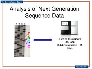
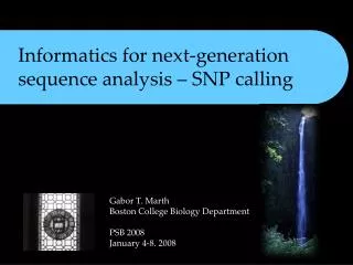
Informatics tools for next-generation sequence analysis. Gabor Marth Boston College Biology Next-Generation Sequencing MiniSymposium CHOP Philadelphia, PA April 6, 2009. New sequencing technologies…. … offer vast throughput. 100 Gb. Illumina/Solexa , AB/ SOLiD sequencers.

E N D
Informatics tools for next-generation sequence analysis Gabor Marth Boston College Biology Next-Generation Sequencing MiniSymposium CHOP Philadelphia, PA April 6, 2009
… offer vast throughput 100 Gb Illumina/Solexa, AB/SOLiD sequencers (10-30Gb in 25-100 bp reads) 10 Gb 1 Gb Roche/454 pyrosequencer (100-400 Mb in 200-450 bp reads) bases per machine run 100 Mb 10 Mb ABI capillary sequencer 1 Mb 10 bp 100 bp 1,000 bp read length
Roche / 454 • pyrosequencing technology • variable read-length • the only new technology with >100bp reads
Illumina / Solexa • fixed-length short-read sequencer • very high throughput • read properties are very close to traditional capillary sequences
AB / SOLiD 2nd Base A C G T 0 1 2 3 A 1 0 3 2 1st Base C 2 3 0 1 G 1 3 2 0 T • fixed-length short-reads • very high throughput • 2-base encoding system • color-space informatics
Helicos / Heliscope • short-read sequencer • single molecule sequencing • no amplification • variable read-length
Many applications • organismal resequencing & de novo sequencing • transcriptome sequencing for transcript discovery and expression profiling Ruby et al. Cell, 2006 Jones-Rhoades et al. PLoS Genetics, 2007 • epigenetic analysis (e.g. DNA methylation) Meissner et al. Nature 2008
Read length 25-60 (variable) 25-50 (fixed) 25-100(fixed) ~200-450 (variable) 400 100 200 300 0 read length [bp]
Coverage bias ~20X read genome read coverage ~2X read genome read coverage
IND (ii) read mapping (iv) SV calling (iii) SNP and short INDEL calling IND (i) base calling (v) data viewing, hypothesis generation The re-sequencing informatics pipeline REF
… and they give you the picture on the box … is like a jigsaw puzzle 2. Read mapping …you get the pieces… Big and Unique pieces are easier to place than others…
Challenge: non-uniqueness • RepeatMasker does not capture all micro-repeats, i.e. repeats at the scale of the read length • Reads from repeats cannot be uniquely mapped back to their true region of origin
Paired-end (PE) reads fragment length: 1 – 10kb fragment length: 100 – 600bp Korbelet al. Science 2007
PE alignment statistics (simulated data) 0.35% 0.00% 7.6% 0.03% 0.09%
The MOSAIK read mapper/aligner Michael Strömberg
Aligning multiple read types together ABI/capillary 454 FLX 454 GS20 Illumina
sequencing error polymorphism Polymorphism detection
Allele calling in multi-individual data -----a----- -----a----- -----c----- -----c----- P(G1=aa|B1=aacc; Bi=aaaac; Bn=cccc) P(G1=cc|B1=aacc; Bi=aaaac;Bn= cccc) P(G1=ac|B1=aacc; Bi=aaaac;Bn= cccc) P(B1=aacc|G1=aa) P(B1=aacc|G1=cc) P(B1=aacc|G1=ac) -----a----- -----a----- -----a----- -----a----- -----c----- Prior(G1,..,Gi,.., Gn) P(Gi=aa|B1=aacc; Bi=aaaac; Bn=cccc) P(Gi=cc|B1=aacc; Bi=aaaac;Bn= cccc) P(Gi=ac|B1=aacc; Bi=aaaac;Bn= cccc) P(Bi=aaaac|Gi=aa) P(Bi=aaaac|Gi=cc) P(Bi=aaaac|Gi=ac) -----c----- -----c----- -----c----- -----c----- P(Bn=cccc|Gn=aa) P(Bn=cccc|Gn=cc) P(Bn=cccc|Gn=ac) P(Gn=aa|B1=aacc; Bi=aaaac; Bn=cccc) P(Gn=cc|B1=aacc; Bi=aaaac;Bn= cccc) P(Gn=ac|B1=aacc; Bi=aaaac;Bn= cccc) “genotype likelihoods” “genotype probabilities” P(SNP)
SNP calling in deep sample sets Allele detection Samples Reads Population
The ability to call rare alleles aatgtagtaAgtacctac aatgtagtaAgtacctac aatgtagtaAgtacctac aatgtagtaAgtacctac aatgtagtaCgtacctac aatgtagtaCgtacctac aatgtagtaAgtacctac aatgtagtaAgtacctac aatgtagtaAgtacctac aatgtagtaAgtacctac aatgtagtaAgtacctac aatgtagtaAgtacctac aatgtagtaAgtacctac aatgtagtaAgtacctac
Detecting de novo mutations • the child inherits one chromosome from each parent • there is a small probability for ade novo (germ-line or somatic) mutation in the child
Targeted mammalian re-sequencing • Deep sequencing of complete human genomes is still too expensive • There is a need to sequence target regions, typically genes, to follow up on GWAS studies • Targeted re-sequencing with • DNA fragment capture offers a • potentially cost-effective alternative • Solid phase or liquid phase capture • 454 or Illumina sequencing • Informatics pipeline must account • for the peculiarities of capture data
On/off target capture ref allele*: 45% non-ref allele*: 54% Target region SNP (outside target region)
Reference allele bias ref allele*: 54% non-ref allele*: 45% (*) measured at 450 het HapMap 3 sites overlapping capture target regions in sample NA07346
SNP example AmitIndap
SV/CNV detection – SNP chips • Tiling arrays and SNP-chips made whole-genome CNV scans possible • Probe density and placement limits resolution • Balanced events cannot be detected
SV/CNV detection – resolution Expected CNVs Karyotype Micro-array Sequencing Relative numbers of events CNV event length [bp]
CNV events found using RD Chromosome 2 Position [Mb]
DNA reference pattern LM LF LM ~ LF+Ldel & depth: low Deletion Ldel Tandemduplication LM ~ LF-Ldup & depth: high Ldup LM ~ LF+LT1LM~ LF+LT2 & depth: normal LM ~ LF-LT1-LT2 LM LM Translocation LT2 LT1 LM LM ~ +Linv & ends flipped LM ~ -Linv depth: normal Inversion Linv un-paired read clusters & depth normal Insertion Lins LM ~LF+LT & depth: normal& cross-paired read clusters Chromosomaltranslocation LT PE read mapping positions
The SV/CNV “event display” Chip Stewart
Data types with standard formats SRF/FASTQ GLF SAM/BAM


![Toward The Next [ Next [ Next … ] ] Generation of Meta-Modeling Tools](https://cdn3.slideserve.com/5854127/toward-the-next-next-next-generation-of-meta-modeling-tools-dt.jpg)