Download
1 / 17
170 likes | 333 Views
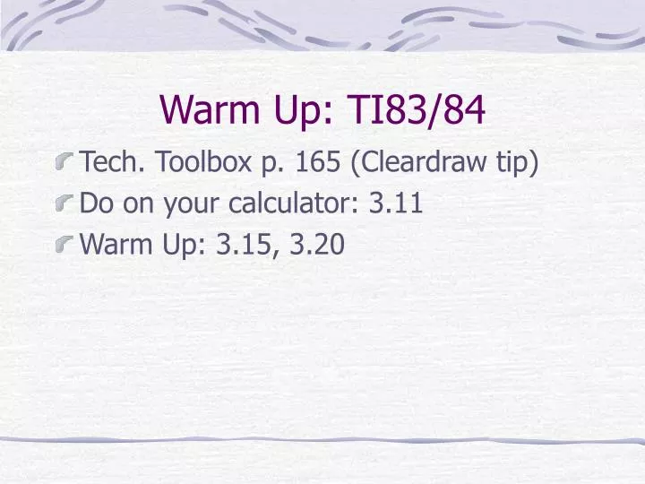
Warm Up: TI83/84. Tech. Toolbox p. 165 (Cleardraw tip) Do on your calculator: 3.11 Warm Up: 3.15, 3.20. 3.2: Least Squares Regression. (LSRL = Least Squares Regression Line) We are required to have an explanatory and response variable.

E N D
Warm Up: TI83/84 • Tech. Toolbox p. 165 (Cleardraw tip) • Do on your calculator: 3.11 • Warm Up: 3.15, 3.20
3.2: Least Squares Regression • (LSRL = Least Squares Regression Line) • We are required to have an explanatory and response variable. • When a scatterplot shows a linear relationship, we summarize the overall pattern by a LSRL; we draw a regression line through the points.
Data: Example 3.9 • Add to L1, L2 • Stat, Calc, 8: Linreg L1, L2, Y1 • Graph with/without YI toggled on • Write down a, b, r, r-squared, y-hat (vital stats)
Interpretation of slope • Slope should be interpreted as predicted or average change in the response variable given a unit change in the explanatory variable. • Carefully graded on AP exam. • Slope is the predicted rate of change in y as x changes. Fat gain = a + b (NEA change) Fat gain = 3.505 – 0.00344 (NEA change) • The slope b = -0.00344 tells us that fat gained goes down by 0.00344 for each added calorie of NEA (x)
Using the LSRL for prediction • Want to predict the fat gain for an individual whose NEA increases by 400 calories when she overeats. • Fat gain = 3.505 – 0.00344 (NEA change) • Fat gain = 3.505 – 0.00344 (400) = 2.13 kgs. • Accuracy depends on how much scatter about the line the data shows (r-squared).
Interpolation = estimating predicted values between known values = GOOD • Extrapolation = usually BAD • Some instances: might be okay to do a “bit” – for example, if you had a strong linear relationship between ages and height and the range of ages from 12 months to 36 months; may be reasonable to extrapolate to 37 months, but not to 60.
Out of all the candidates for the line of best fit (any line we might draw), no other line but the LSRL will produce the smallest possible sum of squared errors. We want a regression line that makes the vertical distances from the line as small as possible. Error = observed–predicted (order is non-negotiable; why – and +) Also called a RESIDUAL
Geometry • The least squares regression line of y on x is the line that makes the sum of the squares of the vertical distances of the data points from the line as small as possible (geometrical interpretation ). • No other regression line would give a smaller sum of squared errors.
Equation of the LSRL • We have data on an explanatory variable x and a response variable y for n individuals. From the data, calculate the means and standard deviations of the 2 variables and their correlation. The LSRL is: with slope Useful property: The point that always passes through the LSRL is (___,___) Therefore the intercept is:
Finding the slope and intercept with formulas • Find x-bar, sx, y-bar, sy, r. • Use formula to find the slope (b). • Use the formula to find a (y-intercept) • Write your LSRL. • Careful – don’t round until the end!
Predicting Values • Find the predicted gain in fat when Non-exercise activity (calories) is 450. • By hand • By Calc
Examining the residuals helps assess how well the line describes the data. • The residual plot makes it easier to study the residuals by plotting them against the explanatory variable. • Magnifies the deviations from the LSRL; makes them easier to see. • Should be no pattern in the residual plot (if no pattern = the LSRL is a good model for the data). • The sum of the residuals is always 0 (special property) • Since the mean of the residuals is always 0, the horizontal line at 0 helps orient us; the residual line (residual = 0) corresponds to the regression line of the original problem.
A few more pointers • The residual plot should show no pattern (curved, straight line, etc.) • Increasing or decreasing spread about the line as x increases indicates that prediction of y will be less accurate for larger x’s • Residuals should be small in size; a LSRL that fits the data well should come close to most of the points. • Standard deviation of the residuals