Download
1 / 48
480 likes | 491 Views
B.1. System of Linear Equations. Equation Solving. A. B. Linear Algebra. Root Finding. linear Multi variable. non-linear Single variable. Open Methods. Brackting Methods. Direct Methods. Iterative Methods. Iterative. Gauss elimination. False- position. Jacobi’s.

E N D
B.1 System of Linear Equations
Equation Solving A B Linear Algebra Root Finding linear Multi variable non-linear Single variable Open Methods Brackting Methods Direct Methods Iterative Methods Iterative Gauss elimination False- position Jacobi’s Bisection Newton- Rapson Gauss-Seidel Gauss- Jordan Secant Choleski’s
Linear Algebraic Equations • An equation of the form ax+by+c=0 or equivalently ax+by=-c is called a linear equation in x and y variables. • ax+by+cz=d is a linear equation in three variables, x, y, and z. • Thus, a linear equation in n variables is a1x1+a2x2+ … +anxn = b • A solution of such an equation consists of real numbers c1, c2, c3, … , cn • If you need to work more than one linear equations, a system of linear equations must be solved simultaneously.
Non-computer Methods for Solving Systems of Equations • For small number of equations (n≤ 3) linear equations can be solved readily by simple techniques such as “graphical method” • Linear algebra provides the tools to solve such a system of linear equations • Nowadays, easy access to computers makes the solution of large sets of linear algebraic equations possible and practical
Solving Small Numbers of Equations • There are many ways to solve a system of linear equations: • Graphical method • Cramer’s rule • Method of elimination • Computer methods
Graphical Method • For two equations: • Solve both equations for x2:
Graphical Method (Contd.) Plot x2 vs. x1 on rectilinear paper, the intersection of the lines gives the solution
Graphical Method (Contd.) No solution Infinite solutions Ill-conditioned (Slopes are too close)
Algebraic Solution Or equate and solve for x1
Cramer’s Rule • Gabriel Cramer was a Swiss mathematician (1704-1752) • Cramer’s rule is another solution technique that is best suited to small numbers of equations
Cramer’s Rule (Contd.) • Each unknown in a system of linear algebraic equations may be expressed as a fraction of two determinants with denominator D and with the numerator obtained from D by replacing the column of coefficients of the unknown in question by the constants b1, b2,... , bn
Coefficient Matrices • Can use determinants to solve a system of linear equations • Use the coefficient matrix of the linear system • Linear System Coefficient Matrix ax+by=e cx+dy=f
Cramer’s Rule for 2x2 System • Let A be the coefficient matrix • Linear SystemCoefficient Matrixax+by=e cx+dy=f If detA 0, then the system has exactly one solution and
Example 1- Cramer’s Rule 2x2 Solve the system: • 8x+5y=2 • 2x-4y=-10 Coefficient matrix is: and
Example 1 (Contd.) Solution: (-1,2)
Example 2- Cramer’s Rule 3x3 • Solve the system: • x+3y-z=1 • -2x-6y+z=-3 • 3x+5y-2z=4 Let’s solve for Z The answer is: (-2,0,1)!!!
System of Linear Equations A set of n equations and n unknowns . . . . . .
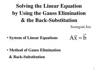
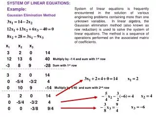
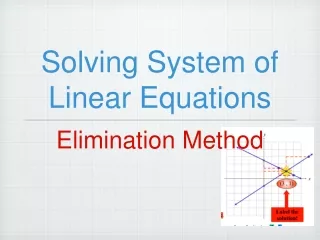
Gaussian Elimination One of the most popular techniques for solving simultaneous linear equations of the form Consists of 2 steps 1. Forward Elimination of Unknowns. 2. Back Substitution
Forward Elimination In general we get:
Forward Elimination At the end of (n-1) Forward Elimination steps, the system of equations will look like: . . . . . .
Back Substitution The goal of Back Substitution is to solve each of the equations using the upper triangular matrix. Example of a system of 3 equations
Back Substitution Start with the last equation because it has only one unknown Solve the second from last equation (n-1)th using xn solved for previously. This solves for xn-1.
Back Substitution Representing Back Substitution for all equations by formula For i=n-1, n-2,….,1 and
Example: Rocket Velocity The upward velocity of a rocket is given at three different times The velocity data is approximated by a polynomial as: Find: The Velocity at t=6,7.5,9, and 11 seconds.
Example: Rocket Velocity Assume Results in a matrix template of the form: Using date from the time / velocity table, the matrix becomes:
Example: Rocket Velocity Forward Elimination: Step 1 Yields
Example: Rocket Velocity Forward Elimination: Step 1 Yields
Example: Rocket Velocity Forward Elimination: Step 2 Yields This is now ready for Back Substitution
Example: Rocket Velocity Back Substitution: Solve for a3 using the third equation
Example: Rocket Velocity Back Substitution: Solve for a2 using the second equation
Example: Rocket Velocity Back Substitution: Solve for a1 using the first equation
Example: Rocket Velocity Solution: The solution vector is The polynomial that passes through the three data points is then:
Example: Rocket Velocity Solution: Substitute each value of t to find the corresponding velocity
Pitfalls Two Potential Pitfalls • Division by zero: May occur in the forward elimination steps. Consider the set of equations: - Round-off error: Prone to round-off errors.
Pitfalls: Example Consider the system of equations: Use five significant figures with chopping = At the end of Forward Elimination =
Pitfalls: Example Back Substitution
Pitfalls: Example Compare the calculated values with the exact solution
Improvements Increase the number of significant digits Decreases round off error Does not avoid division by zero Gaussian Elimination with Partial Pivoting Avoids division by zero Reduces round off error
Partial Pivoting Gaussian Elimination with partial pivoting applies row switching to normal Gaussian Elimination. How? At the beginning of the kth step of forward elimination, find the maximum of If the maximum of the values is In the pth row, then switch rows p and k.
Partial Pivoting What does it Mean? Gaussian Elimination with Partial Pivoting ensures that each step of Forward Elimination is performed with the pivoting element |akk| having the largest absolute value.
Partial Pivoting: Example Consider the system of equations In matrix form = Solve using Gaussian Elimination with Partial Pivoting using five significant digits with chopping
Partial Pivoting: Example Forward Elimination: Step 1 Examining the values of the first column |10|, |-3|, and |5| or 10, 3, and 5 The largest absolute value is 10, which means, to follow the rules of Partial Pivoting, we switch row1 with row1. Performing Forward Elimination
Partial Pivoting: Example Forward Elimination: Step 2 Examining the values of the second column |-0.001| and |2.5| or 0.0001 and 2.5 The largest absolute value is 2.5, so row 2 is switched with row 3 Performing the row swap
Partial Pivoting: Example Forward Elimination: Step 2 Performing the Forward Elimination results in:
Partial Pivoting: Example Back Substitution Solving the equations through back substitution
Partial Pivoting: Example Compare the calculated and exact solution The fact that they are equal is coincidence, but it does illustrate the advantage of Partial Pivoting
Summary • Forward Elimination • Back Substitution • Pitfalls • Partial Pivoting