Download

1 / 16
160 likes | 300 Views
System of Linear Equations. Vivian and Ashley . Linear Demand Functions. Shows the relationship between QUANTITY DEMANDED of the product and PRICE Q D = a – bP ‘a’ = quantity demanded if price is 0 ‘b’ = slope of curve . Example: Change in ‘a’. Q D = 500 – 10P. Q D = 600 – 10P.

E N D
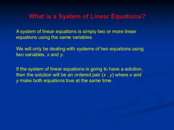
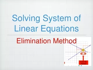
System of Linear Equations Vivian and Ashley
Linear Demand Functions • Shows the relationship between QUANTITY DEMANDED of the product and PRICE • QD= a – bP • ‘a’ = quantity demanded if price is 0 • ‘b’ = slope of curve
Example: Change in ‘a’ QD= 500 – 10P QD= 600 – 10P
Example: Change in ‘b’ QD= 500 – 10P QD= 500 – 20P
Change in ‘b’ =change in slope of the demand curve*CHANGE IN SLOPE IS DIFFERENT FROM CHANGE IN ELASTICITY
Summary • ‘a’ and ‘b’ will be affected by changes in the non-price determinants of demand • Examples of non-price determinants of demand • Income • Price of other products • Tastes/Preferences
Linear Supply Functions • Shows the relationship between QUANTITY SUPPLIED of the product and PRICE • QS= c – dP • ‘c’ = quantity demanded if price is 0 • ‘d’ = slope of curve
Summary • Almost identical to the demand linear function • Change in ‘c’ = parallel shift in curve • Change in ‘d’ = change in slope of the curve
Summary • ‘c’ and ‘d’ will be affected by changes in the non-price determinants of supply • Examples of non-price determinants of supply • The cost of factors of production • The state of technology • Expectations
MARKET EQUILIBRIUM • The intersection between demand curve and supply curve • QD= QS • a – bP = c – dP
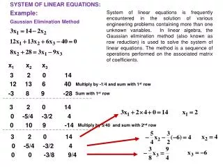
EXAMPLE QD = 2000 – 20P Qs= -400 – 400P
example • QD = 2000 – 200(4) • QD = 1200 units • QS= –400 +400(4) • QS = 1200 units 2000 – 20P = –400 – 400P 2400 = 600P P = $4 or