Download

1 / 21
220 likes | 451 Views
Joint seismic attributes visualization using Self-Organizing Maps . Marcílio Castro de Matos marcilio@ou.edu www.matos.eng.br Kurt J. Marfurt kmarfurt@ou.edu. Motivation: self organizing example. 1- Choosing the attributes. Ex: The ratio between length and width. L. L. W. W.

E N D
Joint seismic attributes visualization using Self-Organizing Maps Marcílio Castro de Matos marcilio@ou.edu www.matos.eng.br Kurt J. Marfurt kmarfurt@ou.edu
Motivation: self organizing example 1- Choosing the attributes Ex: The ratio between length and width L L W W Bananas have high ratio Blueberries have ratio close to one 2- Clustering
Summary • SOM review • SOM 1d • SOM 2d SOM 1d • SOM 2d colormap • SOM3d RGB
Kohonen Self Organizing Maps Input Data: Cartesian coordinates of 3 gaussians centralized in [0,0,0] in red; [3,3,3] in blue and [9,0,0] in green.The “+” signals represent the vectors prototypes. Input DATA MATRIX: 03 attributes with length 3000 13 Winner prototype vector Training neighboohood 7 91 (13x7) prototype vectors
U-matrix Unified Distance Matrix (U-matrix) gives the distances between the neighboring map units. … Red color indicates long distances, and blue color indicates short distances. This U-matrix representation gives an impression of “mountains” (long distances) which divide the map into “fields” (dense parts) or clusters. Each cluster represents different classes.
Clustering of the SOM abstraction Abstraction level1 Abstraction level 22 N samples (input data) M prototype vectors C classes >> >>
2-D source space Attr 2 Pre-image of prototype vectors from target space 1-D target space Class1 Class2 Class3 Attr 1 Kohonen Self Organizing Maps
K-means clusters K-means clustering tend to be attracted to the extreme values and are not ordered in a topological sequence. Kohonen Self Organizing Map SOM-defined classes are in a sequence, so the process is less sensitive to the number of classes (Coleou et al. 2003)
Summary • SOM review • SOM 1d • SOM 2d SOM 1d • SOM 2d colormap • SOM3d RGB
1D Self-Organizing Map12 classes A color equidistant from each other has been got from the HSV circle and has been assigned to each class. It has not been taken into account the distance between the prototype vectors. Classes 0° 30° 60° 90° 120° 150° 180° 210° 240° 270° 300° 330°
1D Self-Organizing Map12 classes The distance among HSV color are proportional to the distance of the prototype vectors. This creates a smoother way to visually the classification result. HSV (Varying Hue, at fixed Saturation and Value) colormap Classes
Principal component projection of the data and the prototype vectors Classes Taking into account the distance among the prototype vectors Classes 0° 30° 60° 90° 120° 150° 180° 210° 240° 270° 300° 330° Don’t taking into account the distance among the prototype vectors
1D Self-Organizing Map256 classes Classes Principal component projection of the data and the prototype vectors
Summary • SOM review • SOM 1d • SOM 2d SOM 1d • SOM 2d colormap • SOM3d RGB
SOM 2D SOM 1D with 16 classes Classes
Classes 1D SOM Classes 2D SOM + 1D SOM
SOM 2D SOM 1D with 256 classes 2D SOM colored prototype vectors and 1D SOM prototype vectors trajectory (white line) Classes
Summary • SOM review • SOM 1d • SOM 2d SOM 1d • SOM 2d colormap • SOM3d RGB
SOM 3D colormap RGB cube The RGB color model mapped to a cube. The horizontal x-axis as red values increasing to the left, y-axis as blue increasing to the lower right and the vertical z-axis as green increasing towards the top. The origin, black, is hidden behind the cube.
Acknowledgements The first two authors would like to thank the support from the University of Oklahoma Attribute-Assisted Seismic Processing and Interpretation Consortium and its sponsors. Attribute-Assisted Seismic Processing and Interpretation http://geology.ou.edu/aaspi/ We also would like to thank PETROBRAS for their cooperation in providing the data, support and the authorization to publish this work.