Download
1 / 19
190 likes | 328 Views
Подход эффективного гамильтониана. 1 . М. С. Лифшиц, ЖЭТФ ( 1957 ). 2 . U.Fano, Phys. Rev. 124, 1866 (1961). 3 . H. Feshbach,, Ann. Phys. (New York) 5 (1958) 357 ; 19 (1962) 287. 4 . C. Mahaux, H.A. Weidenmuller, ( Shell-Model Approach to Nuclear

E N D
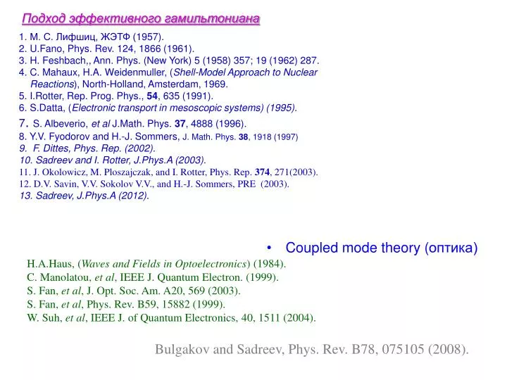
Подход эффективного гамильтониана 1. М. С. Лифшиц, ЖЭТФ (1957). 2. U.Fano, Phys. Rev. 124, 1866 (1961). 3. H. Feshbach,, Ann. Phys. (New York) 5 (1958) 357; 19 (1962) 287. 4. C. Mahaux, H.A. Weidenmuller, (Shell-Model Approach to Nuclear Reactions), North-Holland, Amsterdam, 1969. 5. I.Rotter, Rep. Prog. Phys., 54, 635 (1991). 6. S.Datta, (Electronic transport in mesoscopic systems) (1995). 7. S. Albeverio, et al J.Math. Phys. 37, 4888 (1996). 8. Y.V. Fyodorov and H.-J. Sommers, J. Math. Phys. 38, 1918 (1997) 9. F. Dittes, Phys. Rep. (2002). 10. Sadreev and I. Rotter, J.Phys.A (2003). 11. J. Okolowicz, M. Ploszajczak, and I. Rotter, Phys. Rep. 374, 271(2003). 12. D.V. Savin, V.V. Sokolov V.V., and H.-J. Sommers, PRE (2003). 13. Sadreev, J.Phys.A (2012). • Coupled mode theory (оптика) H.A.Haus, (Waves and Fields in Optoelectronics) (1984). C. Manolatou, et al, IEEE J. Quantum Electron. (1999). S. Fan, et al, J. Opt. Soc. Am.A20, 569 (2003). S. Fan, et al, Phys. Rev. B59, 15882 (1999). W. Suh, et al, IEEE J. of Quantum Electronics, 40, 1511 (2004). Bulgakov and Sadreev, Phys. Rev. B78, 075105(2008).
Coupled defect mode with propagating over waveguide lightManolatou, et al, IEEE J. Quant. Electronics, (1999)
Одно модовый резонатор Coupled mode theory
Инверсия по времени Одно-модовый резонатор CMT • Х. Хаус, Волны и поля в оптоэлектронике
CMT • Много-модовый резонатор IEEE J. Quantum Electronics, 40, 1511 (2004)
Два порта, две моды %CMT for transmission through resonator with two modes clear all E=-2:0.01:2; D=[sqrt(0.1) sqrt(0.25) sqrt(0.1) sqrt(0.25)]; G=0.5*D'*D; H0=diag([-0.25 0.25]); H=H0-1i*G; for j=1:length(E) Q=E(j)*diag([1 1])-H; in=[1; 0]; IN=1i*D'*in; A=Q\IN;; A1(j)=A(1); A2(j)=A(2); t(:,j)=-in+D*A; end
T волновод с двумя резонаторами, Булгаков, Садреев, Phys. Rev. B84, 155304 (2011)
W is matrix NxM where N is the number of eigen states of closed quantum system, M is the number of continuums (channels)
S.Datta, (Electronic transport in mesoscopic systems) (1995).
Проекционные операторы: Уравнение Липпмана-Швингера
S-matrix Basis of closed billiard The biorthogonal basis
c H.-W.Lee, Generic Transmission Zeros and In-Phase Resonances in Time-Reversal Symmetric Single Channel Transport, Phys. Rev. Lett. 82, 2358 (1999)
2d case Limit to continual case
Na=input('input length along transport Na=') Nb=input('input length cross to transport Nb=') Nin=input('input numerical position of the input lead Nin=') Nout=input('input numerical position of the output lead Nout=') NL=length(Nin); NR=length(Nout); vL=1;vR=vL;tb=1; %Leads E=-2.9:0.011:1; HL=zeros(NL,NL); HL=HL-diag(ones(1,NL-1),1); HL=HL+HL'; HL=HL-diag(sum(HL),0); for np=1:NL kpp=acos(-E/2+EL(np,np)/2); kp(np,1:length(E))=kpp; end HR=HL; %Dot N=Na*Nb; HB=zeros(N,N); HB=HB-diag(ones(1,N-1),1)-diag(ones(1,N-Na),Na); HB(Na:Na:N-Na,Na+1:Na:N-Na+1)=0; HB=tb*(HB+HB'); %Coupling matrix psiBin=psiB(Nin,:); psiBout=psiB(Nout,:); WL=vL*psiBin'*psiL'; WR=vR*psiBout'*psiL'; DB=diag(ones(Na*Nb,1)); for j=1:length(E) g=diag(exp(i*kp(:,j))); gg=diag(sin(real(kp(:,j))).^0.5); WW=WL*g*WL'+WR*g*WR'; Heff=diag(EB)-WW; QQ=DB*E(j)-Heff; PP=QQ^(-1); SS=2*i*(WL*gg)'*PP*WR*gg; t(n,j)=SS(1,1); psS=psiB*PP*WL; Matlab calculation
For stationary case l Effective Hamiltonian for time-periodic case
Волновая функция полубесконечного m-го провода N=1
m=-1, 0, 1 21 quasi energies Numerical results N=1 l=0.75, vC=0.25 H. Fukuyama, R. A. Bari, and H.C. Fogedby, PRB (1973). BS, J. Phys. C (1999): Критерий применимости теории возмущений