Confirmatory factor analysis

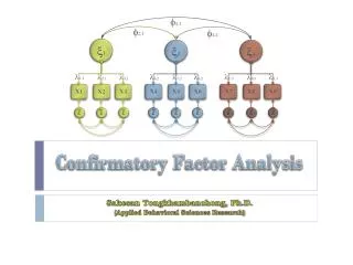
1. Confirmatory factor analysis GHQ 12

3. From Shevlin/Adamson 2005:

4. F1 F2 Model 2 – 2 factor Politi et al, 1994 01 02 03 04 05 06 07 08 09 10 11 12

5. 02 05 06 09 10 11 12 01 03 04 07 08 12 F1 F1 F2 F2 Specifying the model F1 by ghq02* ghq05 ghq06 ghq09 ghq10 ghq11 ghq12; F1@1; F2 by ghq01* ghq03 ghq04 ghq07 ghq08 ghq12; F2@1; F1 with F2;

6. Mplus syntax for ‘model 2’ Variable: Names are ghq01 ghq02 ghq03 ghq04 ghq05 ghq06 ghq07 ghq08 ghq09 ghq10 ghq11 ghq12 f1 id; Missing are all (-9999) ; usevariables = ghq01 ghq03 ghq05 ghq07 ghq09 ghq11 ghq02 ghq04 ghq06 ghq08 ghq10 ghq12; categorical = ghq01 ghq03 ghq05 ghq07 ghq09 ghq11 ghq02 ghq04 ghq06 ghq08 ghq10 ghq12; idvariable = id; Analysis: estimator = WLSMV; model: F1 by ghq02* ghq05 ghq06 ghq09 ghq10 ghq11 ghq12; F1@1; F2 by ghq01* ghq03 ghq04 ghq07 ghq08 ghq12; F2@1; F1 with F2;

7. TESTS OF MODEL FIT Chi-Square Test of Model Fit Value 561.922* Degrees of Freedom 32** P-Value 0.0000 * The chi-square value for MLM, MLMV, MLR, ULSMV, WLSM and WLSMV cannot be used for chi-Square difference tests. MLM, MLR and WLSM chi-square difference testing is described in the Mplus Technical Appendices at www.statmodel.com. See chi-square difference testing in the index of the Mplus User's Guide. ** The degrees of freedom for MLMV, ULSMV and WLSMV are estimated according to a formula given in the Mplus Technical Appendices at www.statmodel.com. See degrees of freedom in the index of the Mplus User's Guide. Chi-Square Test of Model Fit for the Baseline Model Value 9961.631 Degrees of Freedom 13 P-Value 0.0000 CFI/TLI CFI 0.947 TLI 0.978 Number of Free Parameters 50 RMSEA (Root Mean Square Error Of Approximation) Estimate 0.122 WRMR (Weighted Root Mean Square Residual) Value 2.067

8. Results for ‘model 2’ MODEL RESULTS Two-Tailed Estimate S.E. Est./S.E. P-Value F1 BY GHQ02 0.679 0.018 37.113 0.000 GHQ05 0.745 0.015 48.738 0.000 GHQ06 0.816 0.013 61.601 0.000 GHQ09 0.884 0.009 93.445 0.000 GHQ10 0.886 0.009 97.383 0.000 GHQ11 0.845 0.012 68.721 0.000 GHQ12 0.327 0.043 7.516 0.000 F2 BY GHQ01 0.779 0.015 51.337 0.000 GHQ03 0.638 0.021 30.899 0.000 GHQ04 0.737 0.017 44.364 0.000 GHQ07 0.760 0.015 49.694 0.000 GHQ08 0.793 0.016 49.767 0.000 GHQ12 0.516 0.043 11.967 0.000 F1 WITH F2 0.825 0.012 69.584 0.000

9. Results for ‘model 2’ Two-Tailed Estimate S.E. Est./S.E. P-Value Thresholds GHQ01$1 -1.708 0.066 -25.896 0.000 GHQ01$2 0.384 0.038 9.989 0.000 GHQ01$3 1.427 0.055 25.837 0.000 GHQ03$1 -1.246 0.050 -24.816 0.000 GHQ03$2 0.864 0.043 20.076 0.000 GHQ03$3 1.699 0.066 25.922 0.000 GHQ05$1 -1.137 0.048 -23.813 0.000 GHQ05$2 0.154 0.038 4.094 0.000 GHQ05$3 1.213 0.049 24.541 0.000 GHQ07$1 -1.579 0.061 -26.092 0.000 <snip> GHQ12$1 -1.237 0.050 -24.739 0.000 GHQ12$2 0.624 0.040 15.507 0.000 GHQ12$3 1.512 0.058 26.047 0.000 Variances F1 1.000 0.000 999.000 999.000 F2 1.000 0.000 999.000 999.000

10. Graphs

11. Distribution of factors

12. Scatterplot of factors

14. What happened to model 4? WARNING: THE RESIDUAL COVARIANCE MATRIX (THETA) IS NOT POSITIVE DEFINITE. THIS COULD INDICATE A NEGATIVE VARIANCE/RESIDUAL VARIANCE FOR AN OBSERVED VARIABLE, A CORRELATION GREATER OR EQUAL TO ONE BETWEEN TWO OBSERVED VARIABLES, OR A LINEAR DEPENDENCY AMONG MORE THAN TWO OBSERVED VARIABLES. CHECK THE RESULTS SECTION FOR MORE INFORMATION. PROBLEM INVOLVING VARIABLE GHQ03. THE STANDARD ERRORS OF THE MODEL PARAMETER ESTIMATES COULD NOT BE COMPUTED. THE MODEL MAY NOT BE IDENTIFIED. CHECK YOUR MODEL. PROBLEM INVOLVING PARAMETER 39. THE CONDITION NUMBER IS 0.221D-15. FACTOR SCORES WILL NOT BE COMPUTED DUE TO NONCONVERGENCE OR NONIDENTIFIED MODEL.

15. Use tech1 to establish what para-39 is LAMBDA F1 F2 ________ ________ GHQ01 37 0 GHQ03 38 39 GHQ05 0 40 GHQ07 41 0 GHQ09 0 42 GHQ11 43 0 GHQ02 44 0 GHQ04 0 45 GHQ06 46 0 GHQ08 0 47 GHQ10 48 0 GHQ12 0 49 Lambda is the matrix of factor loadings There is a problem with the loading of GHQ03 on the second factor

16. You could actually tell this from the output: MODEL RESULTS Estimate F1 BY GHQ01 0.729 GHQ02 0.660 GHQ03 -1042.356 GHQ06 0.796 GHQ07 0.714 GHQ10 0.868 GHQ11 0.828 F2 BY GHQ03 1042.958 GHQ04 0.692 GHQ05 0.721 GHQ08 0.732 GHQ09 0.859 GHQ12 0.795 F1 WITH F2 1.000 This problem stems from the fact that the third item is loading on both factors. This does not always lead to problems (see other models fitted here) but in this case it has done. It does not appear possible to replicate this model using the current dataset If the aim was not replication, but merely to test one’s own theories, then removing the loading from one of the factors would solve the problem. Depending on your theories on the underlying mechanism, this may or may not be desirable.

17. Conclusions • Based on the level of CFI/TLI, the fit of models 2, 3 and 6 was acceptable (>0.95), however the RMSEA values were too high (> 0.1) • If one were forced to choose between these 3 models, one could argue that model 3 is superior due to parsimony (fewer parameters) and better separation of factors (no double loading) • It is interesting to note that model 3 has the simplest interpretation (pos/neg item wording) whilst model 2 which is subtly different has been given a more theoretical interpretation. • Researchers from different disciplines may interpret the same factor model in different ways – e.g. to support their own theories. It’s a good idea to establish whether you agree with this interpretation.