ELECTROMAGNETICS II

1. ELECTROMAGNETICS II Presented by Dr. SMITA SAMANTA , Professor DEPARTMENT OF ELECTRICAL AND ELECTRONICS ENGINEERING VISAKHA INSTITUTE OF ENGINEERING & TECHNOLOGY

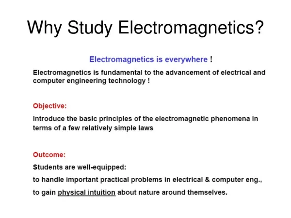
2. Introduction to Electromagnetic Fields • Electromagnetics is the study of the effect of charges at rest and charges in motion. • Some special cases of electromagnetics: • Electrostatics: charges at rest • Magnetostatics: charges in steady motion (DC) • Electromagnetic waves: waves excited by charges in time-varying motion

3. Circuit Theory Introduction to Electromagnetic Fields Maxwell’s equations Fundamental laws of classical electromagnetics Geometric Optics Electro-statics Magneto-statics Electro-magnetic waves Special cases Statics: Transmission Line Theory Input from other disciplines Kirchoff’s Laws

4. Introduction to Electromagnetic Fields • transmitter and receiver • are connected by a “field.”

5. Introduction to Electromagnetic Fields • When an event in one place has an effect on something at a different location, we talk about the events as being connected by a “field”. • A fieldis a spatial distribution of a quantity; in general, it can be either scalar or vector in nature.

6. Introduction to Electromagnetic Fields • Electric and magnetic fields: • Are vector fields with three spatial components. • Vary as a function of position in 3D space as well as time. • Are governed by partial differential equations derived from Maxwell’s equations.

7. Introduction to Electromagnetic Fields • A scalaris a quantity having only an amplitude (and possibly phase). • A vectoris a quantity having direction in addition to amplitude (and possibly phase). Examples: voltage, current, charge, energy, temperature Examples: velocity, acceleration, force

8. Introduction to Electromagnetic Fields • Fundamental vector field quantities in electromagnetics: • Electric field intensity • Electric flux density (electric displacement) • Magnetic field intensity • Magnetic flux density units = volts per meter (V/m = kg m/A/s3) units = coulombs per square meter (C/m2 = A s /m2) units = amps per meter (A/m) units = teslas = webers per square meter (T = Wb/ m2 )

9. Introduction to Electromagnetic Fields • Relationships involving the universal constants: In free space:

10. Introduction to Electromagnetic Fields • Universal constants in electromagnetics: • Velocity of an electromagnetic wave (e.g., light) in free space (perfect vacuum) • Permeability of free space • Permittivity of free space: • Intrinsic impedance of free space:

11. Maxwell’s Equations • Maxwell’s equations in integral form are the fundamental postulates of classical electromagnetics - all classical electromagnetic phenomena are explained by these equations. • Electromagnetic phenomena include electrostatics, magnetostatics, electromagnetostatics and electromagnetic wave propagation. • The differential equations and boundary conditions that we use to formulate and solve EM problems are all derived from Maxwell’s equations in integral form.

12. Maxwell’s Equations • Various equivalence principles consistent with Maxwell’s equations allow us to replace more complicated electric current and charge distributions with equivalent magnetic sources. • These equivalent magnetic sources can be treated by a generalization of Maxwell’s equations.

13. Maxwell’s Equations in Integral Form (Generalized to Include Equivalent Magnetic Sources) Adding the fictitious magnetic source terms is equivalent to living in a universe where magnetic monopoles (charges) exist.

14. Continuity Equation in Integral Form (Generalized to Include Equivalent Magnetic Sources) • The continuity equations are implicit in Maxwell’s equations.

15. S C dS S V dS Contour, Surface and Volume Conventions • open surface S bounded by • closed contour C • dS in direction given by • RH rule • volume V bounded by • closed surface S • dS in direction outward • from V

16. Electric Current and Charge Densities • Jc = (electric) conduction current density (A/m2) • Ji = (electric) impressed current density (A/m2) • qev = (electric) charge density (C/m3)

17. Magnetic Current and Charge Densities • Kc = magnetic conduction current density (V/m2) • Ki = magnetic impressed current density (V/m2) • qmv = magnetic charge density (Wb/m3)

18. Maxwell’s Equations - Sources and Responses • Sources of EM field: • Ki, Ji, qev, qmv • Responses to EM field: • E, H, D, B, Jc, Kc

19. Maxwell’s Equations in Differential Form (Generalized to Include Equivalent Magnetic Sources)

20. Continuity Equation in Differential Form (Generalized to Include Equivalent Magnetic Sources) • The continuity equations are implicit in Maxwell’s equations.

21. Electromagnetic Boundary Conditions Region 1 Region 2

22. Electromagnetic Boundary Conditions

23. Surface Current and Charge Densities • Can be either sources of or responses to EM field. • Units: • Ks - V/m • Js - A/m • qes - C/m2 • qms - W/m2

24. Electromagnetic Fields in Materials • In time-varying electromagnetics, we consider E and H to be the “primary” responses, and attempt to write the “secondary” responses D, B, Jc, and Kcin terms of E and H. • The relationships between the “primary” and “secondary” responses depends on the medium in which the field exists. • The relationships between the “primary” and “secondary” responses are called constitutive relationships.

25. Electromagnetic Fields in Materials • Most general constitutive relationships:

26. Electromagnetic Fields in Materials • In free space, we have:

27. Electromagnetic Fields in Materials • In a simple medium, we have: • linear(independent of field strength) • isotropic(independent of position within the medium) • homogeneous(independent of direction) • time-invariant(independent of time) • non-dispersive (independent of frequency)

28. Electromagnetic Fields in Materials • e = permittivity = ere0 (F/m) • m = permeability = mrm0(H/m) • s = electric conductivity = ere0(S/m) • sm = magnetic conductivity = ere0(W/m)