Download
1 / 40
430 likes | 649 Views
A primer in Biostatistics. Christina M. Ramirez UCLA Department of Biostatistics. Statistics. Data Collection Summarizing Data Interpreting Data Drawing Conclusions from Data. Population.

E N D
A primer in Biostatistics Christina M. Ramirez UCLA Department of Biostatistics
Statistics • Data Collection • Summarizing Data • Interpreting Data • Drawing Conclusions from Data
Population The set of data (numerical or otherwise) corresponding to the entire collection of units about which information is sought Example: Unemployment - Status of ALL employable people (employed, unemployed) in the country.
Sample A subset of the population data that are actually collected in the course of a study. Example: Unemployment - Status of the 1000 employable people interviewed.
Population vs. Sample Population Sample In most studies, it is difficult to obtain information from the entire population. We rely on samples to make estimates or inferences related to the population.
Descriptive statistics Describing data with numbers: measures of location
What to describe? • What is the “location” or “center” of the data? (“measures of location”) • Mean • Median • Mode • How do the data vary? (“measures of variability”) • Range • Interquartile Range • Variant
Mean • Another name for average. • Appropriate for describing measurement data. • Seriously affected by unusual values called “outliers”.
Calculating Sample Mean Add up all of the data points and divide by the number of data points. Example: Number of drinks/day: 2 8 3 4 1 Sample Mean = (2+8+3+4+1)/5 = 3.6
Median • Another name for 50th percentile. • Appropriate for describing measurement data. • “Robust to outliers,” that is, not affected much by unusual values.
Calculating Sample Median Order data from smallest to largest. If odd number of data points, the median is the middle value. Number of drinks/day: 2 8 3 4 1 Ordered Data: 12 3 4 8 Median
Mode • The value that occurs most frequently. • One data set can have many modes. • Appropriate for all types of data, but most useful for categorical data or discrete data with only a few number of possible values. • Example: Number of eyes affected with cataracts in 70 year olds: 0, 1, 2.
The most appropriate measure of location depends on … the shape of the data’s distribution.
Most appropriate measure of location • Depends on whether or not data are “symmetric” or “skewed”. • Depends on whether or not data have one (“unimodal”) or more (“multimodal”) modes.
Choosing Appropriate Measure of Location • If data are symmetric, the mean, median, and mode will be approximately the same. • If data are multimodal, report the mean, median and/or mode for each subgroup. • If data are skewed, report the median.
Descriptive statistics Describing data with numbers: measures of variability Range Interquartile range Variance and standard deviation
Range • The difference between largest and smallest data point. • Highly affected by outliers. • Best for symmetric data with no outliers.
Interquartile range • The difference between the “third quartile” (75th percentile) and the “first quartile” (25th percentile). So, the “middle-half” of the values. • IQR = Q3-Q1 • Robust to outliers or extreme observations. • Works well for skewed data.
Interquartile range Descriptive Statistics Variable N Mean Median TrMean StDev SE Mean GPA 92 3.0698 3.1200 3.0766 0.4851 0.0506 Variable Minimum Maximum Q1Q3 GPA 2.0200 3.9800 2.67253.4675 IQR = 3.4675 - 2.6725 = 0.795
Variance 1. Find difference between each data point and mean. 2. Square the differences, and add them up. 3. Divide by one less than the number of data points.
Variance • If measuring variance of population, denoted by 2 (“sigma-squared”). • If measuring variance of sample, denoted by s2 (“s-squared”). • Measures average squared deviation of data points from their mean. • Highly affected by outliers. Best for symmetric data.
Standard deviation • Sample standard deviation is square root of sample variance, and so is denoted by s. • Units are the original units. • Measures average deviation of data points from their mean. • Also, highly affected by outliers.
Variance or standard deviation Sex N Mean Median TrMean StDev SE Mean female 126 152.05 150.00 151.39 18.86 1.68 male 100 177.98 183.33 176.04 28.98 2.90 Sex Minimum Maximum Q1 Q3 female 108.33 200.00 141.67 163.75 male 125.00 270.00 158.33 197.92 Females: s = 18.86 kph and s2 = 18.862 = 355.7 kph2 Males: s = 28.98 kph and s2 = 28.982 = 839.8 kph2
The most appropriate measure of variability depends on … the shape of the data’s distribution.
Choosing Appropriate Measure of Variability • If data are symmetric, with no serious outliers, use range and standard deviation. • If data are skewed, and/or have serious outliers, use IQR.
Probability The “p” in p-value
Examples: Coin Flips Flips #(Flips) #(Heads) P(H) Ben 4,040 2,048 0.5069 Christina 24,000 12,012 0.5005 Roger 10,000 5,067 0.5067
Probability Concepts Randomness, Independence, Multiplication Rule
Thought Question 1 • What does it mean to say that a deck of cards is “randomly” shuffled? • Every ordering of the cards is equally likely • There are 8 followed by 67 zeros possible orderings of a 52 card deck • Every card has the same probability to end up in any specified location
The question continued • A 52 card deck is randomly shuffled • How often will the tenth card down from the top be a Club? • 1/4 of the time • Every card has the same chance to end up 10th. There are 13 clubs and 13 / 52 = 1/4
More of the question • Deck had three cards - labeled A, B, C • After a random shuffle, cards are turned over one at a time. • How often is the A card the second card that’s turned over? • 1/3 : each card had the same chance to end up in a specific position
Thought Question 2 • A fair die is rolled many times. How often will a “1” be the result? • About 1/6 of the time, but there will be some sampling error • How does increasing the number of rolls affect the difference between sample fraction of “1”’s and 1/6? • Difference likely to get smaller as n increases since margin of error goes down
Does a prior event matter? • A fair coin is flipped four times. • First three flips are heads • What’s the probability that the fourth flip is heads? • 1/2 assuming flips are independent • Results of first three flips don’t matter
Does prior event matter? • Ten cards are drawn without replacement from 52 card deck. • 2 Aces are among these 10 cards • What’s the probability the eleventh card is an Ace? • 2/42 = 1/21 • After ten draws, 42 cards remain, 2 of them are Aces