Download

1 / 48
480 likes | 663 Views
Stratification: Are you a lumper or a splitter?. …and if you are a splitter, how should you split the data and when?. Outline of Stratification Lectures. Definitions, examples and rationale (credibility) Implementation Fixed allocation (permuted blocks) Adaptive (minimization)

E N D
…and if you are a splitter, how should you split the data and when?
Outline of Stratification Lectures • Definitions, examples and rationale (credibility) • Implementation • Fixed allocation (permuted blocks) • Adaptive (minimization) • Rationale - variance reduction • Pre- and post-stratification
Stratification in randomized trials is different from stratified random sampling where the population might be divided up into strata, e.g., census tracts, and each stratum is sampled randomly for some pre-specified sample size.
Typical Situation for Stratification in Trials • Usually, no restriction on number of participants per stratum (goal is to enroll as rapidly as possible and include participants who are representative of target population) • Some trials have goals or put caps on the enrollment of certain subgroups: • ELITE II heart failure trial (Lancet 2000) -- at least 85% of patients had to be > 65 years. • Dietary study to lower BP (DASH) – a target of 50% women and 50% blacks. ,
Stratification • A procedure in which factors known to be associated with the response (prognostic factors) are taken into account in the design (e.g., randomization) • Another type of restriction on the randomization. • Goal of permuted block randomization is to achieve balance on the number in each treatment arm over time. • Goal of stratification is to achieve balance between groups with respect to important prognostic factors. • Pre-stratification refers to a stratified design; post-stratification refers to the analysis
Example: Weight Loss Interventions in Clinical Practice(Appel L et al, N Engl J Med 2011) • 415 participants randomized (1:1:1) to control (n=138), remote support (n=139) or in-person support (n=138) (a modest size trial) • Methods: • “Randomization was stratified according to sex and was generated in blocks of 3 and 6 with use of a Web-based program.” • “The primary analysis was conducted with…repeated measures, mixed-effects. The model included adjustment for clinic, sex , age and race.” • Results: Female sex n=88 in each treatment group
Post-stratification (def.) Classification of experimental units into strata after they have been randomized for the purpose of data analysis e.g., stratified analysis of variance (normally distributed response), Mantel-Haenszel (binary response). Often adjustment for baseline covariates is carried out using regression methods, e.g., linear regression or analysis of covariance (continuous), logistic regression (binary), or Cox regression (time to event) This can be done irrespective of whether you employed pre-stratification. Note: The term post-stratification is sometimes used to describe stratification on data collected post-randomization. Such analyses can be very difficult to interpret. More later on that issue.
General Problems/Issues with Post-Stratification • Model dependence / data dredging • How were covariates (stratifying variables) selected? • How were cut-points (metric) chosen? • Frequently covariates are not pre-specified • Partial solution: Analysis plan in the protocol that includes all covariates considered important (pre-stratification variables + others); updated analysis plan prior to unblinding the results of the study to investigators.
Possible Stratification Scenarios • Pre- plus post-stratification • Pre-stratification only • Post-stratification only • Neither pre- nor post- stratification • Regression adjustment with or without stratification
Advantages • Prevents “accidental bias” resulting from mal-distribution of important prognostic variables • Increases precision (if stratifying variables are related to outcome) • Ensures balance on stratifying factors in early interim analyses (even in large trials) • Facilitates subgroup analysis by stratifyng factor (more optimal allocation ratio) • Results less subject to criticism
International Conference on Harmonization (ICH) Guideline (E-9 Document) “Stratification by important prognostic factors measured at baseline (e.g., severity of disease, age, sex, etc.) may sometimes be valuable in order to promote balanced allocation within strata; this has greater potential benefit in small trials.”
Disadvantages Primarily relates to additional administrative burden of implementation of randomization. • May have several randomization schedules • Measurements to define stratum must be carefully made prior to randomization
What StratificationDoes Not Do 1. Guarantee adequate power to make within-stratum comparisons 2. Eliminate the need to carry out covariate-adjusted analysis • Chance imbalance on other covariates • Analysis consistent with design
Criticisms of UGDP • Definition of target population • Missing data and eligibility errors • Differences in baseline characteristics • “Among the five treatment groups, as well as among clinics, baseline risk factors were also unevenly distributed. This was due to simple randomization of patients without subsequent “stratification” to correct for chance preponderance of antecedent risk factors in one or more of treatment groups.” • Defects in interpretation (e.g., accounting for adherence) Seltzer H, Diabetes 1972 (see also Feinstein A, Clin Pharm Ther 1971 and Biometric Society review, JAMA 1975)
UGDP: Baseline Characteristics Cornfield J, JAMA 1971
Baseline Characteristics of Patients in Trial to Prevent Toxoplasmic Encephalitis(JID 1994;169:384-94) Placebo (n=132) Pyrimethamine (n=264) CD4+ count (cells/mm3) 96.1 97.4 AIDS OI (%)+ 35.2 22.0 Karnofsky Score 89.5 89.7 Hemoglobin (g/dl) 12.6 12.7 + P=0.007
“In view of the major imbalance between the groups in presentation at baseline with AIDS defining OIs, the rigorousness of the allocation procedures need to be supported in detail if the results are to be regarded as credible.” NEJM referee for paper – major reason for rejection
Example How a small difference in an important prognostic variable can bias treatment differences.
Baseline Characteristics in Trial of Didanosine (ddI) and Zalcitabine (ddC)(N Engl J Med 1994; 330:657-662) Age (years) 37.8 8.5 37.5 7.8 CD4+ 75.1 86.2 71.1 84.3 Karnofsky Score 87.2 11.9 85.3 11.9 Prior AIDS 64.8 66.7 Diagnosis (%) ddI (N=230) ddC (N=237) Mean SD Mean SD
Frequency Distribution of Karnofsky Score by Treatment Group ddI ddC < 70 4.8 6.8 70 - 79 10.0 11.8 80 - 89 21.3 24.1 90 - 99 36.1 36.7 100+ 27.8 20.6
Death Rate by Karnofsky Level Death Rate per 100 Person-years < 70 169.8 70 - 79 84.0 80 - 89 41.0 90 - 99 31.9 100+ 18.4 Karnofsky Score
Comparison ofUnadjusted and AdjustedRelative Risk Estimates Unadjusted 0.79 0.11 Adjusted 0.66 0.006 RR (ddC/ddI) P-value
A major problem with this study is the adjustment for the “small differences at baseline” between didanosine and zalcitabine. While there is a “small difference” noted, the variability for each of these variables is quite large. For example, the difference in CD4 count was 4 cells/mm3 between treatment groups; however, the standard error was over 86 cells/mm3. Similarly, for Karnofsky performance status, the difference between the two groups was 2, but the standard error was 11.9. And, finally, there was no difference in the presence of AIDS-defining illness between the two groups. In short, the conclusion that should be drawn is that there is, indeed, no difference between the two groups and attempting to adjust for these small differences is inappropriate. The discussion of Results on page 23, first paragraph, should be eliminated. Comments by NEJM referee – this time no rejection!
Summary • Small differences in a very important prognostic variable (irrespective of significance) can bias treatment comparisons • Large, significant differences in unimportant variables will not bias treatment comparisons • Remember a p-value is a function of both sample size and effect size • Chance imbalances can occur with large sample sizes if there are many strata.
m1A m1B m1 m2A m2B m2 m3A m3B m3 m4A m4B m4 • Typical situation: m1 ≠ m2 ≠ m3 ≠ m4 • Study is designed/powered based on na and nb • Goal: miA = miB for all i. Stratified Design for Comparing Treatments Treatment Stratum A B 1 2 3 4 na nb
Considerations in the Decision to “Lump” or “Split” 1. Size of study 2. Homogeneity of study subjects 3. Strength of prognostic factors (between strata variability) 4. Administrative burden 5. Credibility
Usual Implementation • Block randomization within stratum i.e., prepare a separate randomization schedule for each stratum usually with relatively small block sizes • Makes no sense to use simple randomization Note: The aim of this method is to ensure balance within strata formed by cross-classification of all factor levels.
Typical Stratifying Variables • Clinical site (good idea in multi-center study as each site can be viewed as a replication of study) • Baseline level for outcome of interest • Stage of disease • Combination of factors, e.g., a risk score
Ii π i = 1 Stratification Example: TOMHS • Multi-center (4 clinical sites) trial with two other strata defined by previous use of antihypertensive treatment (Rx) (Yes/No) • 4 x 2 = 8 strata and randomization schedules – aim is to achieve the desired allocation ratio across all 8 groups In general, s stratification variables with Ii levels for the ith variable result in strata. s
One can calculate the probability of obtaining a certain imbalance before the study begins. This can be used to decide whether to stratify the randomization. p(t) is the prob. of randomizing t patients to group A when there are t1 patients in stratum 1. For a certain imbalance one can sum over all p(t) for t's that give that imbalance or worse. ( ) ( ) N N a b p(t) = t t - t 1 ( ) N + N a b t 1
( ) ( ) 100 100 p(t) = t 40 - t ( ) 200 40 Example: Na = 100, Nb = 100, t1 = 40, g = 0.16, h = 0.24 Group A 16 84 100 Group B 24 76 100 Total 40 160 200 Want the prob. of obtaining the imbalance given by g = 0.16, h = 0.24, or worse. Stratum 1 Total Stratum 2 p(t) = 0.216 t ≤ 16 t ≥ 24
Probability of Given Imbalance or More Extreme Total in Stratum FractionAssigned B .52 .48 1.0 .84 .23 .55 .45 .57 .42 .002 .60 .40 .25 .07 – .70 .30 .01 – – FractionAssigned A 1000 100 50
Estimates for the Size of Treatment Imbalance • Let B = block size; K = number of strata; and D = imbalance. • Hallstrom and Davis (Cont Clin Trials, 1988) showed that the total trial imbalance for the number of patients assigned 2 treatments across all strata = D = KB/2 with variance = K(B+1)/6 • Example: Cardiac arrhythmia trial with 270 strata (site, ejection fraction, time since MI) and block size of 4. • Max D = 540; Var (D) = 225; SD (D) = 15; 2 SD = 30. • In this trial, 4200 patients were to be randomized and an imbalance of 30 with probability = 0.05 was considered acceptable.
For small studies with a large number of strata, the use of random permuted blocks within strata can be self-defeating. Example: A study of testicular cancer • 2 treatments • 3 stratifying variables Stage: 2 levels Histology: 3 levels Age: 2 levels No. of strata = 2 x 3 x 2 = 12.
Stage II < 15 ≥ 15 Randomization Schedules for 12 Strata Stage I Histology < 15 ≥ 15 Teratocarcinoma A* A* A* B* A* A* A* A* B A* A* A* A B B B B B B B B B B A Embryonal carcinoma A* B B* A* A* B B* B* B A A B* B A A B* B A B A A B A A Choriocarcinoma B* B A* B* B A B* B* A A B* A A B B* A B B A A A A A B * Patients randomized
Marginal Totals for Strata B A Teratocarcinoma 10 1 Embryonal carcinoma 3 5 Choriocarcinoma 1 6 Stage I 7 1 Stage II 7 11 Age: < 15 8 6 ≥ 15 6 6 TOTAL 14 12
Minimization A method of adaptive stratification which balances the marginal treatment totals for each stratification variable. Interestingly, the European Committee for Proprietary Medicinal Products (CPMP) discourages use of minimization due to concerns about analysis. They note that the methods remain “highly controversial” and are “strongly discouraged”.
References • Taves DR, Clin Pharmacol Ther 1974; 15:443-53. • Pocock S, Simon R. Biometrics 1975; 31:103-15.
Some Notation Let Xik = number of patients already assigned treatment k k = 1, 2 (A or B) for our example i = 1, 2 …, f prognostic factors of a new patient Xtik = Xik if t ≠ k and = Xik+1 if t = k Xtik denotes the new allocation if the new patient is assigned to t. t = 1, 2 (A, B)
(Xti1, Xti2) Lack of Balance Functions B(t) could be a function of Xik or Xtik which measures the “Lack of Balance”: 2 examples Rule of assignment: Use the treatment with smallest B(t) with higher probability. Note: Pocock and Simon’s approach is more general than Taves. It allows for variation among assignments to be considered (e.g., range) and non-deterministic assignment. f B(t) = Xik i = 1 f B(t) = range i = 1
Characteristics of New Patient Example (Pocock, page 85): Number on each treatment Performance status Ambulatory 30 31 x Non-ambulatory 10 9 Age < 50 18 17 x ≥ 50 22 23 Disease-free interval < 2 years 31 32 ≥ 2 years 9 8 x Dominant metastatic Visceral 19 21 x lesion Osseous 8 7 Soft tissue 13 12 Level Factor Patient A B 2 x 2 x 2 x 3 = 24 strata; x denotes the characteristics of the next patient to be randomized. Note: Taves would simply sum marginal totals and randomize to treatment with lowest total. In this case, A(76) instead of B (77).
Estimation of B (1) 1 12 1 11 1 1k 1k i) Factor 1, Level 1 k x x Range (x – x ) 1 30 31 31 – 31 = 0 2 31 31 ii) Factor 2, Level 1 k x x Range (x – x ) 1 18 19 19 - 17 = 2 2 17 17 iii) Factor 3, Level 2 k x x Range (x – x ) 1 9 10 10 – 8 = 2 2 8 8 iv) Factor 4, Level 1 k x x Range (x – x ) 1 19 20 20 – 21 = 1 2 21 21 B (1) = 0 + 2 + 2 + 1 = 5 1 22 1 21 1 2k 2k 1 32 1 31 1 3k 3k 1 42 1 41 1 4k 4k
Estimation of B (2) 2 12 2 11 i) Factor 1, Level 1 k x x Range (x – x ) 1 30 30 30 – 32 = 2 2 31 32 ii) Factor 2, Level 1 k x x Range (x – x ) 1 18 18 18 - 18 = 0 2 17 18 iii) Factor 3, Level 2 k x x Range (x – x ) 1 9 9 9 – 9 = 0 2 8 9 iv) Factor 4, Level 1 k x x Range (x – x ) 1 19 19 19 – 22 = 3 2 21 22 Since B (1) = B (2), toss a coin for the next patient. 2 1k 1k 2 22 2 21 2 2k 2k 2 32 2 31 2 3k 3k 2 42 2 41 2 4k 4k
Implementation Need to continuously update marginal totals to determine B(t) therefore this is best done at a central coordinating/statistical center
Flexibility in allocation: Examples 1. P = 1 if B(1) ≠ B(2) P = 1/2 if B(1) = B(2) Simple randomization if equal, deterministic if unequal 2. P = 2/3 if B(1) ≠ B(2) P = 1/2 if B(1) = B(2) P denotes the: Prob (groups become “more equal”) The more P deviates from 1 when B(1) ≠ B(2), the less effective the balancing
Theoretical Challenge • Not true randomization – in some cases deterministic • Violation of randomization as basis for inference • If the site knows all the margins, then can predict • Reality: When done in a multi-center trial, with central randomization, impossible for sites to predict • Appears random to the sites • Basis for inference: We do inference all the time in non-randomized trials, doesn’t bother us then
Summary • Unless a very small block size is used, over-stratification is likely with use of block randomization within strata if you have many strata relative to the total sample size. • Minimization should be considered for situations where you have several important prognostic factors and a small sample size (particularly if you are concerned about using a very small block size). • Therneau (Cont Clin Trials 1993;14:98-108) suggests that as the number of distinct groups (strata) approaches N/2, adaptive methods be considered.