Download
1 / 60
600 likes | 762 Views
Electrostatics. Electrostatics is the branch of electromagnetics dealing with the effects of electric charges at rest. The fundamental law of electrostatics is Coulomb’s law. Electric Charge.

E N D
Electrostatics • Electrostaticsis the branch of electromagnetics dealing with the effects of electric charges at rest. • The fundamental law of electrostatics is Coulomb’s law. 1
Electric Charge • Electrical phenomena caused by friction are part of our everyday lives, and can be understood in terms of electrical charge. • The effects of electrical charge can be observed in the attraction/repulsion of various objects when “charged.” • Charge comes in two varieties called “positive” and “negative.” 2
Electric Charge • Objects carrying a net positive charge attract those carrying a net negative charge and repel those carrying a net positive charge. • Objects carrying a net negative charge attract those carrying a net positive charge and repel those carrying a net negative charge. • On an atomic scale, electrons are negatively charged and nuclei are positively charged. 3
Electric Charge • Electric charge is inherently quantized such that the charge on any object is an integer multiple of the smallest unit of charge which is the magnitude of the electron charge e= 1.602 10-19C. • On the macroscopic level, we can assume that charge is “continuous.” 4
Coulomb’s Law • Coulomb’s law is the “law of action” between charged bodies. • Coulomb’s law gives the electric force between two point chargesin an otherwise empty universe. • A point charge is a charge that occupies a region of space which is negligibly small compared to the distance between the point charge and any other object. 5
Coulomb’s Law Q1 Q2 Unit vector in direction of R12 Force due to Q1 acting on Q2 6
Coulomb’s Law • The force on Q1due to Q2 is equal in magnitude but opposite in direction to the force on Q2 due to Q1. 7
Qt Q Electric Field • Consider a point charge Q placed at the origin of a coordinate system in an otherwise empty universe. • A test charge Qtbrought near Qexperiences a force: 8
Electric Field • The existence of the force on Qt can be attributed to an electric field produced by Q. • The electric field produced by Q at a point in space can be defined as the force per unit charge acting on a test charge Qtplaced at that point. 9
Electric Field • The basic units of electric field are newtons per coulomb. • In practice, we usually use volts per meter. 10
Continuous Distributions of Charge • Charge can occur as • point charges (C) • volume charges (C/m3) • surface charges (C/m2) • line charges (C/m) most general 11
Electrostatic Potential • An electric field is a force field. • If a body being acted on by a force is moved from one point to another, then workis done. • The concept of scalar electric potential provides a measure of the work done in moving charged bodies in an electrostatic field. 12
b a q Electrostatic Potential • The work done in moving a test charge from one point to another in a region of electric field: 13
C Electrostatic Potential • The electrostatic field is conservative: • The value of the line integral depends only on the end points and is independent of the path taken. • The value of the line integral around any closed path is zero. 14
Electrostatic Potential • The work done per unit charge in moving a test charge from point a to point b is the electrostatic potential difference between the two points: electrostatic potential difference Units are volts. 15
Electrostatic Potential • Since the electrostatic field is conservative we can write 16
Electrostatic Potential • Thus the electrostatic potentialV is a scalar field that is defined at every point in space. • In particular the value of the electrostatic potential at any point P is given by reference point 17
Electrostatic Potential • The reference point (P0) is where the potential is zero (analogous to ground in a circuit). • Often the reference is taken to be at infinity so that the potential of a point in space is defined as 18
Electrostatic Potential and Electric Field • The work done in moving a point charge from point a to pointb can be written as 19
Electrostatic Potential and Electric Field • Along a short path of length Dl we have 20
Electrostatic Potential and Electric Field • Along an incremental path of length dlwe have • Recall from the definition of directional derivative: 21
Electrostatic Potential and Electric Field • Thus: the “del” or “nabla” operator 22
Visualization of Electric Fields • An electric field (like any vector field) can be visualized using flux lines (also called streamlinesor lines of force). • A flux line is drawn such that it is everywhere tangent to the electric field. • A quiver plot is a plot of the field lines constructed by making a grid of points. An arrow whose tail is connected to the point indicates the direction and magnitude of the field at that point. 23
Visualization of Electric Potentials • The scalar electric potential can be visualized using equipotential surfaces. • An equipotential surface is a surface over which V is a constant. • Because the electric field is the negative of the gradient of the electric scalar potential, the electric field lines are everywhere normal to the equipotential surfaces and point in the direction of decreasing potential. 24
charged sphere (+Q) + + + metal + insulator Faraday’s Experiment 25
Faraday’s Experiment (Cont’d) • Two concentric conducting spheres are separated by an insulating material. • The inner sphere is charged to +Q. Theouter sphere is initially uncharged. • The outer sphere is groundedmomentarily. • The charge on the outer sphere is found to be -Q. 26
Faraday’s Experiment (Cont’d) • Faraday concluded there was a “displacement” from the charge on the inner sphere through the inner sphere through the insulator to the outer sphere. • The electric displacement (or electric flux) is equal in magnitude to the charge that produces it, independent of the insulating material and the size of the spheres. 27
+Q -Q Electric Displacement (Electric Flux) 28
Electric (Displacement) Flux Density • The density of electric displacement is the electric (displacement) flux density, D. • In free space the relationship between flux density and electric field is 29
Electric (Displacement) Flux Density (Cont’d) • The electric (displacement) flux density for a point charge centered at the origin is 30
Gauss’s Law • Gauss’s law states that “the net electric flux emanating from a close surface S is equal to the total charge contained within the volume V bounded by that surface.” 31
S ds V Gauss’s Law (Cont’d) By convention, ds is taken to be outward from the volume V. Since volume charge density is the most general, we can always write Qencl in this way. 32
Applications of Gauss’s Law • Gauss’s law is an integral equation for the unknown electric flux density resulting from a given charge distribution. known unknown 33
Applications of Gauss’s Law (Cont’d) • In general, solutions to integral equations must be obtained using numerical techniques. • However, for certain symmetric charge distributions closed form solutions to Gauss’s law can be obtained. 34
Applications of Gauss’s Law (Cont’d) • Closed form solution to Gauss’s law relies on our ability to construct a suitable family of Gaussian surfaces. • A Gaussian surface is a surface to which the electric flux density is normal and over which equal to a constant value. 35
V S Gauss’s Law in Integral Form 36
V S Recall the Divergence Theorem • Also called Gauss’s theorem or Green’s theorem. • Holds for any volume and corresponding closed surface. 37
Applying Divergence Theorem to Gauss’s Law Because the above must hold for any volume V, we must have Differential form of Gauss’s Law 38
The Need for Poisson’s and Laplace’s Equations (Cont’d) • Poisson’s equation is a differential equation for the electrostatic potential V. Poisson’s equation and the boundary conditions applicable to the particular geometry form a boundary-value problem that can be solved either analytically for some geometries or numerically for any geometry. • After the electrostatic potential is evaluated, the electric field is obtained using 39
Derivation of Poisson’s Equation • For now, we shall assume the only materials present are free space and conductors on which the electrostatic potential is specified. However, Poisson’s equation can be generalized for other materials (dielectric and magnetic as well). 40
Derivation of Poisson’s Equation (Cont’d) Poisson’s equation 2 is the Laplacian operator. The Laplacian of a scalar function is a scalar function equal to the divergence of the gradient of the original scalar function. 42
Laplacian Operator in Cartesian, Cylindrical, and Spherical Coordinates 43
Laplace’s Equation • Laplace’s equation is the homogeneous form of Poisson’s equation. • We use Laplace’s equation to solve problems where potentials are specified on conducting bodies, but no charge exists in the free space region. Laplace’s equation 44
Uniqueness Theorem • A solution to Poisson’s or Laplace’s equation that satisfies the given boundary conditions is the unique (i.e., the one and only correct) solution to the problem. 45
Fundamental Laws of Electrostatics in Integral Form Conservative field Gauss’s law Constitutive relation 46
Fundamental Laws of Electrostatics in Differential Form Conservative field Gauss’s law Constitutive relation 47
Fundamental Laws of Electrostatics • The integral forms of the fundamental laws are more general because they apply over regions of space. The differential forms are only valid at a point. • From the integral forms of the fundamental laws both the differential equations governing the field within a medium and the boundary conditions at the interface between two media can be derived. 48
Boundary Conditions • Within a homogeneous medium, there are no abrupt changes in E or D. However, at the interface between two different media (having two different values of e), it is obvious that one or both of these must change abruptly. 49
Boundary Conditions (Cont’d) • To derive the boundary conditions on the normal and tangential field conditions, we shall apply the integral form of the two fundamental laws to an infinitesimally small region that lies partially in one medium and partially in the other. 50