Download

1 / 45
500 likes | 750 Views
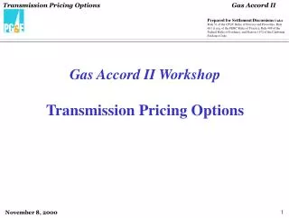
Gas transmission pricing models for entry-exit systems. 6th Annual CRNI Conference, Brussels November 22 – 2013 Bert Kiewiet. Contents.

E N D
Gas transmission pricing models for entry-exit systems 6th Annual CRNI Conference, Brussels November 22 – 2013 Bert Kiewiet
Contents This paper discusses the major gas transmission pricing models. It explains how they allocate costs to entry/exit points. It assesses the applicability to network topologies. Four cost allocation models Main objectives of tariff design Application of four models to two networks Introduction to entry-exit systems Conclusions Gas Transmission Pricing Models and Implementation Options
Introduction / The Entry-Exit System The functionality of the entry-exit system is explained using a schematical representation. X N System boundary Contractual flow of gas Physical exit point Physical entry point Source: DNV KEMA 2013 – Entry-exit regimes in gas available on: http://ec.europa.eu/energy/gas_electricity/studies/gas_en.htm
Introduction / The Entry-Exit System One of the main features is that network users contract entry and exit capacity separately. Network users can contract entry and exit capacity separately.
Introduction / The Entry-Exit System Another feature is that gas which has entered the system can be nominated to any off-take point. Gas brought into the system at any entry point can be made available for off-take at any exit point within the system on a fully independent basis, without any restrictions
Introduction / The Entry-Exit System The virtual point is a fundamental feature of the entry-exit model. It facilitates the bilateral title transfer of gas between network users. The virtual trading point offers the users the possibility to bilaterally transfer title of gas and/or swap imbalances between network users.
Introduction / The Entry-Exit System Ideally the shipper books the exit capacity only at the network level where final exit takes place. Network users only book exit capacity on the level where the final exit takes place. Imbalances between injections and withdrawals are aggregated across all entry and exit points in a network user’s portfolio, regardless of the network level.
Introduction / The Entry-Exit System The functionality of the entry-exit system is explained using a schematical representation. X N System boundary Contractual flow of gas Physical exit point Physical entry point Source: DNV KEMA 2013 – Entry-exit regimes in gas available on: http://ec.europa.eu/energy/gas_electricity/studies/gas_en.htm
Introduction / EU Regulations The entry-exit systems is the mandatory access model for gas transmission system operators in the European Union. Regulation provides overall requirements for tariffs. Regulation (EC) no. 715/2009: • Implementation of the entry-exit system is mandatory in the European Union. • Tariff setting in the entry-exit model: • Tariffs should be set separately for every entry and exit point • Tariffs should not be calculation on the basis of contract paths • Non-discrimination between domestic transport and transit • Member States developed different solutions. • Harmonisation: • ACER: Framework guidelines regarding harmonised transmission tariffs structures • ENTSOG: Development of a network code on harmonised tariff structures (to do)
Main Objectives Of Tariff Setting The Third Energy Package specifies objectives for the setting of tariffs. Experience shows that other, more practical, aspects are important also. Third Energy Package objectives: • Cost reflectivity • Non-discrimination • Avoid cross-subsidisation • Economic efficiency • Cost recovery • Transparency Practical requirements: • Stability and predictability • Stakeholder acceptance • Efficient regulation • Macro-economic constraints
Entry 1 Entry 1 Entry 1 Cost Allocation Models Applied To Two Networks Exit 1 Exit 1 Entry 2 Cost allocation models address the issue of different ways to allocate the allowed revenue to the specific entry and exit points. Four models are applied to two networks. Exit 1 Entry 2 Exit 3 Exit 3 Exit 2 Exit 2 Cost allocation Transit network Ring shaped network Entry 2 Postage stamp Entry 3 Entry 3 Exit 2 Matrix Exit 3 Distance to Virtual Point Capacity Weighted Distance
Different Keys For Allocation Of Costs To Entry-Exit Points Cost allocation models address the issue of different ways to allocate the allowed revenue to the specific entry and exit points. Four models are applied to two networks. Cost allocation Some features Postage stamp • Most straightforward. • Single uniform tariff, does not provide locational signals • Likely to involve cross subsidies between network users. • Not particularly suitable for networks with longer distances Matrix • Uses replacement cost as a key to allocate revenue • Optimisation problem: additional constraints can easily be applied.
Different Keys For Allocation Of Costs To Entry-Exit Points Cost allocation models address the issue of different ways to allocate the allowed revenue to the specific entry and exit points. Four models are applied to two networks. Cost allocation Some features Distance to Virtual Point • Uses distance as a key to allocate costs • Based on the assumption that tariffs should reflect the costs of bringing gas to the virtual point. • Takes into account the direction of the flow under peak conditions. Negative distances = cost savings. • Resulting tariffs provide locational signals. Capacity Weighted Distance • Uses distance as a key to allocate costs as well. • Additional weighing by technical capacities of the entry and exit points.
1. Setting of Allowed Revenue 2. Allocation of Cost to Entry or Exit points Postage Stamp – calculation steps The postage stamp is the most straightforward of all cost allocation methodologies. It does not provide any locational signals. It is less suitable for long distance networks. Steps: Features: • Single uniform tariff applied to either the entry or exit points • Does not provide any locational signals • Not particularly suitable for transmission networks with longer distances • Likely to involve cross subsidies between network users due to the uniform tariff level • Starting point of the tariff calculation • Set by regulator • Costs are allocated to entry and exit points in proportion to the booked capacity • Results in a uniform tariff for all points
1. Setting of Allowed Revenue 2. Allocation of Cost to Pipeline Sections 3. Derivation of Entry-Exit Tariffs 4. Supplementary Adjustments Matrix approach – calculation steps The matrix approach used replacement costs of sections as a key for the allocation of revenues. Steps: • Starting point of the tariff calculation • Set by regulator • Allocation of allowed revenue to different pipeline sections (external key for allocation: replacement costs of sections) • Derivation of unit cost by incorporating chargeable capacity • Construction of unit cost matrix. • Calculation of tariffs by minimizing differences between unit costs and entry-exit tariffs. • Tariffs adjustments to meet the requirements of being competitive, sustainable and affordable to network users and ensuring a successful transition.
Cost Allocation Models Applied To Two Networks Cost allocation models address the issue of different ways to allocate the allowed revenue to the specific entry and exit points. The models are applied to two networks. Cost allocation General calculation approach Postage stamp • Basic starting point is the allowed revenue • Arbitrarily chosen value for the allowed revenue • Focus is on the revenue allocation question • Only capacity charges are considered (EUR/kWh/day/year) Matrix Distance to Virtual Point Capacity Weighted Distance
Entry 1 = 97 GWh/day Entry 1 Entry 1 = 360 GWh/day Cost Allocation Models Applied To Two Networks Entry 2 =170 GWh/day Exit 1 Exit 1 Cost allocation models address the issue of different ways to allocate the allowed revenue to the specific entry and exit points. The models are applied to two networks. Exit 1 = 3 GWh/day Entry 2 Exit 3 Exit 3 Exit 2 Exit 2 Transit network Ring shaped network Entry 2 = 5 GWh/day Entry 3 = 97 GWh/day Entry 3 Exit 2 = 2 GWh/day Exit 3 = 360 GWh/day
Results Transit Network The four cost allocation models were applied to the transit network. The resulting (capacity) tariffs for the entry and exit points are presented.
Results Transit Network The four cost allocation models were applied to the transit network. The resulting (capacity) tariffs for the entry and exit points are presented. The main entry and exit point are priced similarly for each model. The main entry and exit point are priced
Results Transit Network The four cost allocation models were applied to the transit network. The resulting (capacity) tariffs for the entry and exit points are presented. In the distance to virtual point the exits closest to the main entry point is priced lowest: • Value of chosen cost driver (total distance) is lower.
Results Transit Network The four cost allocation models were applied to the transit network. The resulting (capacity) tariffs for the entry and exit points are presented. This effect is also observed in the capacity weighted distance model (though less pronounced): • In CWD this effect is lessened by the capacity as additional cost driver.
Results Transit Network The four cost allocation models were applied to the transit network. The resulting (capacity) tariffs for the entry and exit points are presented. The trend is different in the matrix approach: • Both spur lines have same dimensions, but exit 2 has lower bookings unit cost higher.
Entry 1 = 97 GWh/day Entry 1 Entry 1 = 360 GWh/day Cost Allocation Models Applied To Two Networks Entry 2 =170 GWh/day Exit 1 Exit 1 Cost allocation models address the issue of different ways to allocate the allowed revenue to the specific entry and exit points. The models are applied to two networks. Exit 1 = 3 GWh/day Entry 2 Exit 3 Exit 3 Exit 2 Exit 2 Transit network Ring shaped network Entry 2 = 5 GWh/day Entry 3 = 97 GWh/day Entry 3 Exit 2 = 2 GWh/day Exit 3 = 360 GWh/day
Results Ring Shaped Network The four cost allocation models were applied to the ring shaped network. The resulting (capacity) tariffs for the entry and exit points are presented
Results Ring Shaped Network The four cost allocation models were applied to the ring shaped network. The resulting (capacity) tariffs for the entry and exit points are presented Tariffs of distance to virtual point = postage stamp: • Due to symmetry in network topology. • Distance to virtual point does not take into account differences in booked capacities.
Results Ring Shaped Network The four cost allocation models were applied to the ring shaped network. The resulting (capacity) tariffs for the entry and exit points are presented On the entry side the capacity weighted distance model = distance to virtual point model: • Booked capacities at exit points are equal to each other. • Network symmetry and thus equal distances.
Results Ring Shaped Network The four cost allocation models were applied to the ring shaped network. The resulting (capacity) tariffs for the entry and exit points are presented Exit 3 is priced highest: • Furthest away from entry with highest booked capacity
Results Ring Shaped Network The four cost allocation models were applied to the ring shaped network. The resulting (capacity) tariffs for the entry and exit points are presented Matrix approach results in opposite outcomes: • Exit tariffs are similar (booked capacity is same) • Thus difference in booked capacity is now solely reflected in entry tariffs.
Results Ring Shaped Network The four cost allocation models were applied to the ring shaped network. The resulting (capacity) tariffs for the entry and exit points are presented Tariff entry 2is lower: • Due to higher booked capacity at entry 2 (lower unit costs). • This effect discourages the use of the other entry points (undesired effect).
Concluding Remarks We have demonstrated four cost allocation models for calculating network tariffs. Results differ due to algorithms applied and the chosen cost drivers. • For all four models the basic starting point is the allowed revenue of the network operator. Postage stamp model: • Generally, the postage stamp model may be suitable in highly meshed networks where models resulting in locationally different tariffs might be too cumbersome • Application of equal tariffs does not affect cost-reflectivity too much • Additionally relevant when tariff equality is prioritized over other principles Distance to virtual point: • Distance as key for cost allocation • Takes into account direction of the flow Capacity weighted distance model: • Distance as key for cost allocation • Capacity weighing
Concluding Remarks We have demonstrated four cost allocation models for calculating network tariffs. Results differ due to algorithms applied and the chosen cost drivers. Matrix approach: • Replacement cost as key to allocate revenues • Allows for an easy incorporation of additional pricing considerations, for example: • Equity requirements • Transition needs, and • Price stability General: • The models are just different mathematical ways to describe reality and largely aim to achieve the same. • Results differ due to differences in the algorithms applied and in particularly the chosen cost drivers. • Trade-offs between the complexity of the model and its outcome • More complex networks may require more detailled modelling • Unilateral networks could be represented by less sophisticated modelling efforts
Contact Bert KIEWIET Senior Consultant Markets & Regulation Management & Operating Consulting KEMA Nederland B.V. Energieweg 17, 9743 AN Groningen P.O. Box 2029, 9704 CA Groningen The Netherlands www.dnvkema.com Bert.Kiewiet@dnvkema.com Tel: +31 50 700 98 69 Fax: +31 50 700 98 59
Derivation of Entry-Exit Tariffs Entry Exit Each pipeline section has its own replacement value Stylized network: C F B Exit Entry A E G D Exit Example of applying the replacement value of pipeline sections to distribute the Allowed Revenue to be recovered by the various sections
Derivation of Entry-Exit Tariffs Unit cost matrix: Exit D Exit F Exit G UCAB+UCBD Entry A UCAB+UCBE + UCEF UCAB+UCBE + UCEG Entry C UCCB+UCBD UCCB+UCBE + UCEF UCCB+UCBE + UCEG Tariffs: Exit D Exit F Exit G TariffAB+ TariffBD Entry A TariffAB + TariffEF TariffAB+ TariffEG TariffCB+ TariffBD Entry C TariffCB+ TariffEF TariffCB + TariffEG Unit cost matrix can be constructed by applying the shortest-path method Tariffs from one network point to another (entry tariff + exit tariff) should equal (as much as possible) the unit costs of this route
Derivation of Entry-Exit Tariffs • Values for sum of the entry and exit tariffs need to the same as the corresponding values of the unit cost matrix (cannot be solved algebraically) • This can be achieved by applying an Least Squares approach which results in the following minimization task: • min ∑ij (Cij – (TNi + TXj))2 • This minimization problem can be solved by using a numerical solver (for example using Excel’s Solver) • Usually, additional adjustments are necessary to attain the eventual tariffs: • Scaling to the required revenue • Incorporation of the main objectives in tariff setting (equity goals, stability and predictability, transparency, etc.)
1. Setting of Allowed Revenue 2. Calculate flows and direction in network 3. Calculate distance to reference node 4. Calculating tariff Distance To Virtual Point The distance to the virtual point is based on the assumption that the entry and exit tariffs should reflect the costs of bringing gas to the virtual point. Steps: • Starting point of the tariff calculation • Set by regulator • Definition of network sections • Calculateflows at peak demandsituation. • Determine flow directions • Reference node canbearbitrarilychosen • Calculatedistancefromeach point toreference node • Distances may be negative (cost savings) • Tariff = distance * constant unit cost of infrastructure • Scalingtariffs in order toreachallowedrevenue
Distance To Virtual Point The distance to the virtual point is based on the assumption that the entry and exit tariffs should reflect the costs of bringing gas to the virtual point. Features: • Costs are allocatedto the different entry and exit points based on the distanceto the virtual point (reference node). • The reference node canbearbitrarilychosen. • Resultingtariffsprovidelocationalsignals.
1. Setting of Allowed Revenue 2. Create a distance matrix 3. Calculate capacity weighted distance 4. Calculate tariffs Capacity Weighted Distance Uses distance as a key to allocate costs as well, but weighs them with the technical capacities of the demand/supply node. Steps: • Starting point of the tariff calculation • Set by regulator • Create a matrix with the distances between every entry point and exit point. • Calculate the proportion of the capacity of each entry/exit point relativeto the totalcapacity • Calculate capacity weighted distance for each entry point and exit point. • Multiplydistanceby the share of capacity exit j in reltaiontototal exit capacity • For each point the revenue recovered is calculated. • Dividing the revenue per point and the booked capacity yields the tariff
Entry Exit C F B Exit Entry A E G D Exit Operational costs € / year Capitalcosts€ / year Return on assets€ / year + Allowed revenue € / year
Entry Exit C F B Exit Entry A E G D Exit Allowed revenue € / year Booked capacity kWh/day/year
D11 D1j D = Dl1 DIJ AD
Different keys for allocation of costs to entry-exit points x Postage stamp model: • Single uniform tariffappliedtoeither the entry or exit points • Does notprovideanylocationalsignals • Likelytoinvolve cross subsidies betweennetworkusers dueto the uniform tarifflevel • Notparticularlysuitablefor transmission networkswithlongerdistances Distanceto Virtual Point Model: • Usesdistance as a keytoallocatecosts • Takes into account the direction of the flow under peak conditions CapacityWeightedDistance Model: • Usesdistance as a keytoallocatecosts as well, but weighsthemwith the technicalcapacities of the demand/supply node Matrix Approach • Usesreplacementcost as a key (andthusimplicitlyassumeslength/diameter as major cost drivers
Matrix approach The matrix approach used replacement costs of sections as a key for the allocation of revenues. Features: • Replacementcosts of sectionsused as keyforallocation of revenue bearssomesimilaritywithmarginalcost pricing. • Calculation of unit costs per segment: • Low utilisation of sectionsmay lead tohigher unit costsforthatsection. May result in signalsoppositetowhatwouldbedesired. • Alternatively a marginalcost concept canbeapplied. This approach willrequireadditionaladjustments t ensurerevenue recovery. • Sincethis is anoptimisationproblem, additionalconstraintscanbeapplied.