Download
1 / 16
190 likes | 209 Views
Data analysis with R and the tidyverse. Jean-Fred Fontaine Steffen Albrecht March 2019. fontaine@uni-mainz.de s.albrecht@uni-mainz.de. The course. Objectives Powerful data analysis and visualization from little programming skills R and the tidyverse R: core statistical software

E N D
Data analysis with R and the tidyverse Jean-Fred Fontaine Steffen Albrecht March 2019 fontaine@uni-mainz.de s.albrecht@uni-mainz.de
The course • Objectives • Powerful data analysis and visualization from little programming skills • R and the tidyverse • R: core statistical software • Tidyverse: extensions to R + more readable code • Schedule on 2 days • Brief introduction and overview of the basics • Tutorial on the tidyverse • More exercises and additional functions
Preparation • Install and open R Studio • Download the data files • https://cbdm.uni-mainz.de/mb19/ • Download and decompress the folder datasets_danalysis.zip in your user directory • Set the R’s “working directory” to the decompressed folder named datasets • From the Menu Session / Set Working Directory / Choose Directory • Install packages tidyverse and ggvis in R Studio • From the menu: Tools / Install Packages … • Or from the console: install.packages(c("tidyverse ", "ggvis"))
R Studio interface Variables Source code or data tables Files, plots or help (F1) R console
Tips • The # symbol indicates to R that what follows is a comment • Commands are separated by a new line • Lists, piped commands and content within parentheses or brackets can be spread over different lines • Parentheses and brackets must be closed • R is case sensitive # LOAD LIBRARY library(tidyverse) # LOAD AND DISPLAY TABLE column_names <- c("probe_id", "expression", "present") cd103minus <- read_tsv( "file.tsv", col_names=column_names ) cd103minus %>% select(probe_id, expression) %>% head()
Tips • Some keyboard shortcuts • [TAB] for text auto-completion of function or object names • [CTRL]+[ENTER] to run the selected lines from the code editor to the console • [ALT]+[-] to insert assignment symbols (<-) • [CTRL]+[SHIFT]+[m] to insert the pipe symbols (%>%) • In the console, use arrow keys to traverse through the history of commands • "Up arrow" – traverse backwards (older commands) • "Down arrow" – traverse forward (newer commands)
as calculator • Simple operations • 1+3 # will return 4 • Statistical functions • sqrt(81) # will the square root of 81 that is 9 • 1 + abs(-4) # will return absolute value of -4 plus 1 = 5 • The Order of Operations • Do calculations inside Parentheses first • 6 × (5 + 3) = 6 × 8 = 48 • Then compute Exponents (Powers, Roots) before multiplication and division • 5 × 22= 5 × 4 = 20 • Then Multiply or Divide (before you Add or Subtract) • 2 + 5 × 3 = 2 + 15 = 17 • Otherwise just go left to right
Objects and variables • R stores everything in objects having defined types • Some common object types • numeric (e.g. 1, 25.5, 1e-6) • character (e.g. “ABCD”, “Hello World 24!”) • logical (TRUE or T, FALSE or F, NA for not applicable)) • factor: categorical values (numeric index associated to character labels) • vector: used to store a set of objects • function: (e.g. library, abs, sqrt) • Variables • Names to remember and reuse objects • x <- 2 # variable x is assigned value 2 • The class function returns the type • class(x) # R returns "numeric" • class("ABC") # R returns “character"
Vectors # Vector of 4 numeric objects x <- c(1.2, # 1st object 2.3, # 2nd object 0.2, # 3rd object 1.1) # 4th object # Indexing some values X # 1.2 2.3 0.2 1.1 x[1] # 1.2 x[ length(x) ] # 1.1 x[3] # 0.2 x[ c(2,3,4) ] # 2.3 0.2 1.1 x[ 2:4 ] # 2.3 0.2 1.1
Tables • Several types of tables • matrix - table of objects of the same type • data.frame - table of objects of same or different types • tibble – extension of data.frame for working with large tables • tibbles have a refined print method (default few rows and columns fit screen) • each column reports its type • numerics may be detailed as integers (int) or double precision values (dbl)
TABLE [ ROW, COL ] TABLE$COL[ ROW ] Tables df <- data_frame( x = 1:5, y = 1, z = x^2+y ) df # A tibble: 5 x 3 x y z <int> <dbl> <dbl> 1 1 1 2 2 2 1 5 3 3 1 10 4 4 1 17 5 5 1 26 df[1,1] # 1 df[1,2] # 1 df[1,3] # 2 df[1,] # 1 1 2 df[1,3] # 2 df[2,3] # 5 df[,3] # 2 5 10 17 26 df$z# 2 5 10 17 26 df[ 4:5 , 1:2 ] # A tibble: 2 x 2 x y <int> <dbl> 1 4 1 2 5 1
FOR LOOPS # Vector of character objects x <- c("file1.csv", # 1st object "file2.csv", # 2nd object "file3.csv") # 3rd object # Looping on some values for(my_file in x){ text <- paste("We have", my_file) print(text) } [1] "We have file1.csv" [1] "We have file2.csv" [1] "We have file3.csv"
LOGICAL OPERATIONS 1<2 # TRUE ! (1<3) # FALSE (logical NOT: !) 1 != 3 # TRUE (3 != 1) & (2 >= 1.9) # TRUE (logical AND: &) (3 == 1) | (3 < 5) # TRUE (logical OR: |) y <- c(TRUE, FALSE, 5>2) Y # TRUE FALSE TRUE
For more details see help pages Some useful functions • Table statistics • rownames(x) • colnames(x) • dim(x) – number of rows and columns • summary(x) – summary statistics • Table join / merge • left_join() • full_join() • rbind() – add rows (base R) • cbind() – add columns (base R) • Statistics • length(x) • max(x) • min(x) • sum(x) • mean(x) • median(x) • var(x) • sd(x) • cor() – correlation coefficient • t.test() – Student’s t-test • Other • seq() – sequence of numbers
Tidyverse Tutorial https://cbdm.uni-mainz.de/mb19/ Gregorio Alanis has created the tutorial but works now elsewhere. Please email only your current teachers for questions: fontaine@uni-mainz.de s.albrecht@uni-mainz.de