Download
1 / 102
1.04k likes | 1.49k Views
Introduction to Pattern Recognition for Human ICT Review of probability and statistics. 2014. 9. 19 Hyunki Hong. Contents. Probability Random variables Random vectors The Gaussian random variable. Review of probability theory. • Definitions (informal)

E N D
Introduction to Pattern Recognition for Human ICTReview of probability and statistics 2014. 9. 19 Hyunki Hong
Contents • Probability • Random variables • Random vectors • The Gaussian random variable
Review of probability theory • Definitions (informal) 1. Probabilities are numbers assigned to events that indicate “how likely” it is that the event will occur when a random experiment is performed. 2. A probability law for a random experiment is a rule that assigns probabilities to the events in the experiment. 3. The sample space S of a random experiment is the set of all possible outcomes. • Axioms of probability 1. Axiom I: 𝑃[𝐴𝑖] ≥ 0 2. Axiom II: 𝑃[𝑆] = 1 3. Axiom III: 𝐴𝑖∩𝐴j= ∅ ⇒ 𝑃[𝐴𝑖 ⋃ 𝐴𝑗] = 𝑃[𝐴𝑖] + 𝑃[𝐴𝑗]
More properties of probability 예) N=3, P[A1] + P[A2] + P[A3] - P[A1∩A2] - P[A1∩A3] - P[A2∩A3] +P[A1∩A2∩A3]
Conditionalprobability • If A and B are two events, the probability of event A when we already know that event B has occurred is 1. This conditional probability P[A|B] is read: – the “conditional probability of A conditioned on B”, or simply – the “probability of A given B” • Interpretation 1. The new evidence “B has occurred” has the following effects. - The original sample space S (the square) becomes B (the rightmost circle). - The event A becomes A∩B. 2. P[B] simply re-normalizes the probability of events that occur jointly with B.
Theorem of total probability • Let 𝐵1, 𝐵2, …, 𝐵𝑁be a partition of 𝑆 (mutually exclusive that add to 𝑆). • Any event 𝐴 can be represented as 𝐴 = 𝐴∩𝑆 = 𝐴∩(𝐵1∪𝐵2 …𝐵𝑁) = (𝐴∩𝐵1)∪(𝐴∩𝐵2)…(𝐴∩𝐵𝑁) • Since 𝐵1, 𝐵2, …, 𝐵𝑁are mutually exclusive, then 𝑃[𝐴] = 𝑃[𝐴∩𝐵1] + 𝑃[𝐴∩𝐵2] + ⋯ + 𝑃[𝐴∩𝐵𝑁] and, therefore 𝑃[𝐴] = 𝑃[𝐴|𝐵1]𝑃[𝐵1]+ ⋯ + 𝑃[𝐴|𝐵𝑁] 𝑃[𝐵𝑁] =
Bayes theorem • Assume {𝐵1, 𝐵2, …, 𝐵𝑁}is a partition of S • Suppose that event 𝐴 occurs • What is the probability of event 𝐵𝑗? • Using the definition of conditional probability and the theorem of total probability we obtain • This is known as Bayes Theorem or Bayes Rule, and is (one of) the most useful relations in probability and statistics.
Bayes theorem & statistical pattern recognition • When used for pattern classification, BT is generally expressed as where 𝜔𝑗is the 𝑗-th class (e.g., phoneme) and 𝑥 is the feature/observation vector (e.g., vector of MFCCs) • A typical decision rule is to choose class 𝜔𝑗with highest P[𝜔𝑗|𝑥]. Intuitively, we choose the class that is more “likely” given observation 𝑥. • Each term in the Bayes Theorem has a special name 1. 𝑃[𝜔𝑗]prior probability (of class 𝜔𝑗) 2. 𝑃[𝜔𝑗|𝑥]posterior probability (of class 𝜔𝑗given the observation 𝑥) 3. 𝑝[𝑥|𝜔𝑗]likelihood (probability of observation 𝑥 given class 𝜔𝑗) 4. 𝑝[𝑥]normalization constant (does not affect the decision) Mel-frequency cepstrum (MFC): 단구간 신호의 파워스펙트럼을 표현하는 방법. 비선형적인 Mel스케일의 주파수 도메인에서 로그파워스펙트럼에 cosine transform으로 얻음. Mel-frequency cepstral coefficients (MFCCs)는 여러 MFC들을 모아 놓은 계수들을 의미함. (음성신호처리)
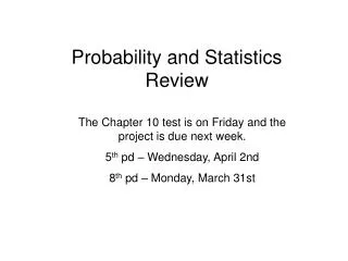
Example 1. Consider a clinical problem where we need to decide if a patient has a particular medical condition on the basis of an imperfect test. - Someone with the condition may go undetected (false-negative). - Someone free of the condition may yield a positive result (false-positive). 2. Nomenclature - The true-negative rate P(NEG|-COND) of a test is called its SPECIFICITY - The true-positive rate P(POS|COND) of a test is called its SENSITIVITY 3. Problem - Assume a population of 10,000 with a 1% prevalence for the condition - Assume that we design a test with 98% specificity and 90% sensitivity - Assume you take the test, and the result comes out POSITIVE - What is the probability that you have the condition? 4. Solution - Fill in the joint frequency table next slide, or - Apply Bayes rule TN / (TN+FP) X 100 특이도 민감도 TP / (TP+FN) X 100
198 9,702
Random variables • When we perform a random experiment, we are usually interested in some measurement or numerical attribute of the outcome. ex) weights in a population of subjects, execution times when benchmarking CPUs, shape parameters when performing ATR • These examples lead to the concept of random variable. 1. A random variable 𝑋 is a function that assigns a real number 𝑋(𝜉)to each outcome 𝜉 in the sample space of a random experiment. 2. 𝑋(𝜉)maps from all possible outcomes in sample space onto the real line.
Random variables • The function that assigns values to each outcome is fixed and deterministic, i.e., as in the rule “count the number of heads in three coin tosses” 1. Randomness in 𝑋 is due to the underlying randomness of the outcome 𝜉 of the experiment • Random variables can be 1. Discrete, e.g., the resulting number after rolling a dice 2. Continuous, e.g., the weight of a sampled individual
Cumulative distribution function (cdf) • The cumulative distribution function 𝐹𝑋(𝑥) of a random variable 𝑋 is defined as the probability of the event {𝑋 ≤ 𝑥} 𝐹𝑋(𝑥) = 𝑃[𝑋 ≤ 𝑥] − ∞ < 𝑥 < ∞ • Intuitively, 𝐹𝑋(𝑏)is the long-term proportion of times when 𝑋(𝜉)≤ 𝑏. • Properties of the cdf
Probability density function (pdf) • The probability density function 𝑓𝑋(𝑥) of a continuous random variable 𝑋, if it exists, is defined as the derivative of 𝐹𝑋(𝑥). • For discrete random variables, the equivalent to the pdf is the probability mass function • Properties
Statistical characterization of random variables • The cdf or the pdf are SUFFICIENT to fully characterize a r.v. • However, a r.v. can be PARTIALLY characterized with other measures • Expectation (center of mass of a density) • Variance (spread about the mean) • Standard deviation • N-th moment
Random vectors • An extension of the concept of a random variable 1. A random vector 𝑋is a function that assigns a vector of real numbers to each outcome 𝜉 in sample space 𝑆 2. We generally denote a random vector by a column vector. • The notions of cdf and pdf are replaced by ‘joint cdf’ and ‘joint pdf’. 1. Given random vector 𝑋 = [𝑥1, 𝑥2, …, 𝑥𝑁]𝑇we define the joint cdf as 2. and the joint pdf as • The term marginal pdf is used to represent the pdf of a subset of all the random vector dimensions 1. A marginal pdf is obtained by integrating out variables that are of no interest ex) for a 2D random vector 𝑋= [𝑥1, 𝑥2]𝑇, the marginal pdf of 𝑥1 is
Statistical characterization of random vectors • A random vector is also fully characterized by its joint cdf or joint pdf. • Alternatively, we can (partially) describe a random vector with measures similar to those defined for scalar random variables. • Mean vector: • Covariance matrix
• The covariance matrix indicates the tendency of each pair of features (dimensions in a random vector) to vary together, i.e., to co-vary 1. The covariance has several important properties – If 𝑥𝑖and 𝑥𝑘tend to increase together, then 𝑐𝑖𝑘> 0 – If 𝑥𝑖tends to decrease when 𝑥𝑘increases, then 𝑐𝑖𝑘< 0 – If 𝑥𝑖and 𝑥𝑘are uncorrelated, then 𝑐𝑖𝑘=0 – |𝑐𝑖𝑘 | ≤ 𝜎𝑖𝜎𝑘, where 𝜎𝑖is the standard deviation of 𝑥𝑖. – 𝑐𝑖𝑖= 𝜎𝑖2 = 𝑣𝑎𝑟[𝑥𝑖] 2. The covariance terms can be expressed as 𝑐𝑖𝑖= 𝜎𝑖2 and 𝑐𝑖𝑘=𝜌𝑖𝑘𝜎𝑖𝜎𝑘. – where 𝜌𝑖𝑘is called the correlation coefficient.
A numerical example • Given the following samples from a 3D distribution 1. Compute the covariance matrix. 2. Generate scatter plots for every pair of vars. 3. Can you observe any relationships between the covariance and the scatter plots? 4. You may work your solution in the templates below. 2 2 4 -2 -2 0 4 4 0 4 0 0 3 4 6 -1 0 2 1 0 4 0 -2 0 5 4 2 1 0 -2 1 0 4 0 -2 0 6 6 4 2 2 0 4 4 0 4 0 0 4 4 4 0 0 0 2.5 2 2 2 -1 0
The Normal or Gaussian distribution • The multivariate Normal distribution 𝑁(𝜇,Σ) is defined as • For a single dimension, this expression is reduced to
• Gaussian distributions are very popular since 1. Parameters 𝜇,Σ uniquely characterize the normal distribution 2. If all variables 𝑥𝑖are uncorrelated (𝐸[𝑥𝑖𝑥𝑘] = 𝐸[𝑥𝑖]𝐸[𝑥𝑘]), then – Variables are also independent (𝑃[𝑥𝑖𝑥𝑘] = 𝑃[𝑥𝑖]𝑃[𝑥𝑘]), and – Σ is diagonal, with the individual variances in the main diagonal. • Central Limit Theorem (next slide) • The marginal and conditional densities are also Gaussian. • Any linear transformation of any 𝑁 jointly Gaussian r.v.’s results in 𝑁 r.v.’s that are also Gaussian. 1. For 𝑋 = [𝑋1𝑋2…𝑋𝑁]𝑇jointly Gaussian, and 𝐴𝑁×𝑁invertible, then 𝑌 = 𝐴𝑋 is also jointly Gaussian.
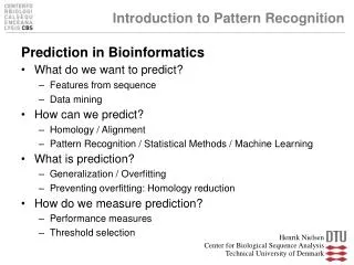
• Central Limit Theorem 1. Given any distribution with a mean 𝜇 and variance 𝜎2, the sampling distribution of the mean approaches a normal distribution with mean 𝜇 and variance 𝜎2/𝑁 as the sample size 𝑁 increases - No matter what the shape of the original distribution is, the sampling distribution of the mean approaches a normal distribution. - 𝑁 is the sample size used to compute the mean, not the overall number of samples in the data. 2. Example: 500 experiments are performed using a uniform distribution. - 𝑁 = 1 1) One sample is drawn from the distribution and its mean is recorded (500 times). 2) The histogram resembles a uniform distribution, as one would expect. - 𝑁 = 4 1) Four samples are drawn and the mean of the four samples is recorded (500 times) 2) The histogram starts to look more Gaussian - As 𝑁 grows, the shape of the histograms resembles a Normal distribution more closely.
01_기초 통계 • 통계학 • 자료를 정보화하고 이를 바탕으로 하여 객관적인 의사 결정 과정을 연구하는 학문 • 불확실한 상태 추정의 문제 • 불확실한 상태의 판별 및 분석을 위한 방법으로 확률적인 여러 기법들 사용 • Ex: 노이즈가 심한 데이터모델링 및 분석 • 패턴인식에서는 통계학적인 기법들을 이용하여 주어진 상태에 대한 통계 분석이 필수 • 확률값을 이용한 상태 추정 • 확률: 개연성, 신뢰도, 발생 빈도 등..
01_기초 통계 • 통계 용어 • 추정 • 요약된 데이터를 기반으로 특정 사실을 유도해 내는 것 • 데이터 분석의 신뢰성 • 서로 다르게 반복적으로 데이터를 수집하더라도 항상 동일한 결과가 얻어지는가? • 즉, 보편적인 재현이 가능한가? • 모집단 • 데이터 분석의 관심이 되는 전체 대상 • 표본 • 모집단의 특성을 파악하기 위해서 수집된 모집단의 일부분인 개별 자료 • 표본 분포 • 동일한 모집단에서 취한, 동일한 크기를 갖는 가능한 모든 표본으로부터 얻어진 통계 값들의 분포
01_기초 통계 • 통계 파라미터 • 평균(mean) • 자료의 총합을 자료의 개수로 나눈 값. • 자료 분포의 무게 중심에 해당한다. • 분산(variance) • 평균으로 부터 자료가 흩어져 있는 정도. • 자료로부터 평균값의 차이에 대한 제곱 값. • 표준 편차(standard deviation) • 분산의 제곱근을 취하여 자료의 차수(1차) 와 일치시킨 것을 말한다.
01_기초 통계 • 바이어스(bias) • 데이터의 편향된 정도를 나타냄
01_기초 통계 • 공분산(covariance) • 두 종류 이상의 데이터가 주어질 경우에 두 변수사이의 연관 관계에 대한 척도 • 표본 데이터 이변량 데이터(bivariate) 일 경우의 공분산 계산 • Ex xi: 2시~3시 사이에 아트센터 정문을 출입하는 사람의 수 yi: 2시~3시 사이의 평균 기온 • 변수들 간의 선형관계가 서로 정방향(+)인지 부방향(-)인지 정도만 나타냄. Cov(x, y) > 0 : 정방향 선형관계 Cov(x, y) < 0 : 부방향 선형관계 Cov(x, y) = 0 : 선형관계가 없음
01_기초 통계 • 상관 계수(correlation coefficient) • 두 변량 X,Y 사이의 상관관계의 정도를 나타내는 수치(계수) • 공분산과의 차이점: • 공분산: 변수들 간의 선형관계가 정방향인지부방향인지 정도만 나타냄. • 상관 계수: 선형 관계가 얼마나 밀접한지를 나타내는 지표 • 변수들의 분포 특성과는 관계 없음.
01_기초 통계 • Ex: 도서관 상주시간, 성적, 결석횟수의 상관관계 • 작은 상관 계수는 선형적으로 두 성분간의 관련성이 거의 없음을 나타낸다. • 음의 상관 계수는 두 성분이 서로 상반되는 특성을 가짐을 의미함. x1: 주당 도서관에 있는 시간 x2: 패턴인식 과목 점수 x3: 주당 결석 시간
01_기초 통계 • 왜도(skewness, skew) • 분포가 어느 한쪽으로 치우친(비대칭:asymmetry) 정도를 나타내는 통계적 척도. • 오른쪽으로 더 길면 양의 값이 되고 왼쪽으로 더 길면 음의 값이 된다. • 분포가 좌우 대칭이면 0이 된다.
01_기초 통계 • 첨도(kurtosis) • 뾰족한(peakedness) 정도를 나타내는 통계적 척도이다.
2차원 데이터 생성 • 특정 확률분포를 따라 확률적으로 생성 • 연구 목적에 맞는 데이터 확률분포 정의 • 이 분포로부터 랜덤하게 데이터 추출 • 균등분포 rand() • 가우시안 분포 randn() 일반적인 경우 평균/공분산에 따른 변환 필요
2차원 데이터 생성 replicate and tile an array N=25; m1=repmat([3,5], N,1); m2=repmat([5,3], N,1); s1=[1 1; 1 2]; s2=[1 1; 1 2]; X1=randn(N,2)*sqrtm(s1)+m1; X2=randn(N,2)*sqrtm(s2)+m2; plot(X1(:,1), X1(:,2), '+'); hold on; plot(X2(:,1), X2(:,2), 'd'); save data2_1 X1 X2; matrix square root normally distributed pseudorandom numbers ex) Generate values from a normal distribution with mean 1 and stadard deviation 2 r = 1+2.*randn(100,1)
2차원 데이터 생성 1 1 2 2 학습 데이터 테스트 데이터
1 m1 2 m2 학습 : 데이터의 분포 특성 분석 • 분포 특성 분석 결정경계 load data2_1; m1 = mean(X1); m2 = mean(X2); s1 = cov(X1); s2 = cov(X2); save mean2_1 m1 m2 s1 s2; 학습 데이터로부터 추정된 평균과 공분산
분류 : 결정경계의 설정 • 판별함수 d(m1,xnew)-d(m2,xnew)=0 • 클래스 라벨 xnew C1 d(m1,xnew) m1 d(m2,xnew) m2 C2
성능 평가 load data2_1; load mean2_1 Etrain=0; N=size(X1,1) for i=1:N d1=norm(X1(i,:)-m1); d2=norm(X1(i,:)-m2); if (d1-d2) > 0 Etrain = Etrain+1; end d1=norm(X2(i,:)-m1); d2=norm(X2(i,:)-m2); if (d1-d2) < 0 Etrain = Etrain+1; end end fprintf(1,'Training Error = %.3f\n', Etrain/50); • 학습 오차 계산 프로그램
성능 평가 2/50 3/50 학습 데이터 테스트 데이터
데이터의 수집과 전처리 0 1 2 3 4 5 6 7 8 9 0 1 2 3 4 5 6 7 8 9 0 1 2 3 4 5 6 7 8 9 0 1 2 3 4 5 6 7 8 9 0 1 2 3 4 5 6 7 8 9 0 1 2 3 4 5 6 7 8 9 0 1 2 3 4 5 6 7 8 9 테스트 데이터 전처리를 거친 데이터 집합 (크기 정규화, 이진화) 학습 데이터 수집된 데이터 집합
데이터 변환 영상데이터를 읽어 데이터 벡터로 표현하고 저장 • (전처리된)영상 데이터(20x16) 벡터(320차원) for i=0:1:9 for j=3:7 fn = sprintf('digit%d_%d.bmp', i, j); xi = imread(fn); x = reshape(double(xi), 20*16, 1); Xtrain(:, i*5+j-2) = x; Ttrain(i*5+j-2, 1) = i; end for j=1:2 fn = sprintf('digit%d_%d.bmp', i, j); xi = imread(fn); x = reshape(double(xi), 20*16, 1); Xtest(:, i*2+j) = x; Ttest(i*2+j, 1) = i; end end save digitdataXtrainTtrainXtestTtest 학습 데이터 320x50 reshape array: 320 by 1 학습데이터집합: 320 by50 클래스 레이블: 320 by50 테스트 데이터 320x20
학습과 결정경계 load digitdata for i=0:1:9 mX(:, i+1) = mean(Xtrain(:, i*5+1:i*5+5)’)’; end save digitMeanmX; mXi = uint8(mX*255); for i = 0:1:9 subplot(1, 10, i+1); imshow(reshape(mXi(:, i+1), 20, 16)); end • 학습 데이터에 대한 평균 벡터 계산 convert to unsigned 8-bit integer 평균영상 결정규칙
분류와 성능 평가 결정규칙 load digitdata; load digitMean Ntrain = 50; Ntest = 20; Etrain = 0; Etest = 0; for i = 1:50 x = Xtrain(:.i); for j = 1:10 dist(j) = norm(x - mX(:, j)); end [minv, minc_train(i)] = min(dist); if(Ttrain(i) ~= (minc_train(i) - 1)) Etrain = Etrain+1; end end for i = 1:20 x = Xtest(:, i); for j = 1:10 dist(j) = norm(x - mX(:, j)); end [minv, minc_test(i)] = min(dist); if(Ttest(i) ~= (minc_test(i) - 1)) Etest = Etest+1; end end 학습 데이터 minv: 최소값. minc_train: 최소거리를 갖는 평균 영상데이터 레이블 테스트 데이터
분류와 성능 평가 테스트 데이터 (오차 15%) 학습 데이터 (오차 2%)
01_기초 통계 • 회귀분석 • 회귀직선 • 표본 집합을 대표하는 최적의 직선을 구하는 과정 • 각 표본에서 직선까지의 거리 합이 가장 작은 직선을 구하는 과정 • 각 표본에서 직선에 내린 수선의 길이의 제곱 값의 합이 최소인 직선을 구함 • '최소 자승법(Method of Least Mean Squares, LMS)'
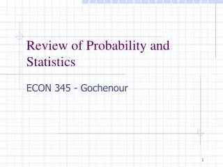
Least squares line fitting • Data: (x1, y1), …, (xn, yn) • Line equation: yi = m xi + b • Find (m, b) to minimize y=mx+b (xi, yi) Normal equations: least squares solution to XB = Y
예제(선형대수학) • Data: (x1, y1), …, (xn, yn) • Line equation: yi = m xi + b, y1= m x1+ b, …, yn= m xn+ b 위 식으로 얻어진 y = m x + b • (0, 1), (1, 3), (2, 4), (3, 4)의 최소제곱직선? 측정오차있으면, 측정된 점은 직선 위에 있지 않음. : 최소제곱직선(least squares line of best fit) 또는 회귀직선(regression line)
Total least squares • Distance between point (xi, yi) and line ax+by=d (a2 + b2 = 1): |axi + byi – d| • Find (a, b, d) to minimize the sum of squared perpendicular distances ax+by=d Unit normal: N=(a, b) (xi, yi)
Total least squares Solution to (UTU)N = 0, subject to ||N||2 = 1: eigenvector of UTUassociated with the smallest eigenvalue (least squares solution to homogeneous linear systemUN = 0) second moment matrix