Download
1 / 31
400 likes | 795 Views
Summary Statistics. Last week we used stemplots and histograms to describe the shape , location , and spread of a distribution. This week we use numerical summaries of location and spread. Main Summary Statistics by Type. Central location Mean Median Mode Spread

E N D
Summary Statistics Last week we used stemplots and histograms to describe the shape, location, and spread of a distribution. This week we use numerical summaries of location and spread. Summary Statistics
Main Summary Statistics by Type • Central location • Mean • Median • Mode • Spread • Variance and standard deviation • Quartiles and Inter Quartile Range (IQR) • Shape • Statistical measures of spread (e.g., skewness and kurtosis) are available but are seldom used in practice (not covered) Summary Statistics
Notation • n sample size • X variable • xi value of individual i • sum all values (capital sigma) • Illustrative example (sample.sav), data: 21 42 5 11 30 50 28 27 24 52 • n= 10 • X = age • x1= 21, x2= 42, …, x10= 52 • x = 21 + 42 + … + 52 = 290 Summary Statistics
Sample Mean Illustrative example: n = 10 (data & intermediate calculations on prior slide) Summary Statistics
Population Mean • Same operation as sample mean, but based on entire population (N = population size) • Not available in practice, but important conceptually Summary Statistics
Interpretation of xbar • Sample mean used to predict • an observation drawn at random from a sample • an observation drawn at random from the population • the population mean • Gravitational center (balance point) Summary Statistics
Median – a different kind of average • “Middle value” • Covered last week • Order data • Depth of median is (n+1) / 2 • When n is odd middle value • When n is even average two middle values • Illustrative example, n = 10 median has depth (10+1) / 2 = 5.5 05 11 21 24 27 28 30 42 50 52median = average of 27 and 28 = 27.5 Summary Statistics
Outlier Median is “robust” Robust resistant to skews and outliers This data set has a mean (xbar) of 1600: 1362 1439 1460 1614 1666 1792 1867 This data set has an outlier and a mean of 2743: 1362 1439 1460 1614 1666 1792 9867 The median is 1614 in both instances. The median was not influenced by the outlier. Summary Statistics
Mode • Mode value with greatest frequency • e.g., {4, 7, 7, 7, 8, 8, 9} has mode = 7 • Used only in very large data sets Summary Statistics
Mean, Median, Mode • Symmetrical data: mean = median • positive skew: mean > median [mean gets “pulled” by tail] • negative skew: mean < median Summary Statistics
Spread = Variability • Variability amount values spread above and below the average • Measures of spread • Range and inter-quartile range • Standard deviation and variance (this week) Summary Statistics
Range = max – min The range is rarely used in practice b/c it tends to underestimate population range and is not robust Summary Statistics
Deviation = Sum of squared deviations = Sample standard deviation = Standard deviation Most common descriptive measure of spread Sample variance = Summary Statistics
Standard deviation (formula) Sample standard deviation s is the unbiased estimator of population standard deviation . Population standard deviation is rarely known in practice. Summary Statistics
New data set (“Metabolic Rates”)This example is not in your lecture notes Metabolic rates (cal/day), n = 7 1792 1666 1362 1614 1460 1867 1439 Summary Statistics
Metabolic rates showing mean (*) and deviations of first two observations Summary Statistics
Standard Deviation Calculationmetabolic.sav – introduced slide 15 * Sum of deviations will always equal zero Summary Statistics
Standard Deviation Metabolic data (cont.) Variance (s2) Standard deviation (s) Summary Statistics
General rule for rounding means and standard deviations • Report mean to one additional decimals above that of the data • To achieve accuracy, intermediate calculations should carry still an additional decimals • Illustrative example • Suppose data is recorded with one decimal accuracy (i.e., xx.x) • Report mean with two decimal accuracy (i.e., xx.xx) • Carry all intermediate calculations with at least three decimal accuracy (i.e., xx.xxx) Even more important: Always use common sense and judgment. Summary Statistics
TI-30XIIS – about $12 In practice, we often use software or a calculator to check our standard deviation Summary Statistics
Interpretation of Standard Deviation • Larger standard deviation greater variability • s1 = 15 and s2 = 10 group 1 has more variability • 68-95-99.7 rule – Normal data only • 68% of data with 1 SD of mean, 95% within 2 SD from mean, and 99.7% within 3 SD of mean • e.g., if mean = 30 and SD = 10, then 95% of individuals are in the range 30 ± (2)(10) = 30 ± 20 = (10 to 50) • Chebychev’s rule – All data • at least 75% data within 2 SD of mean • e.g., mean = 30 and SD = 10, then at least 75% of individuals in range 30 ± (2)(10) = (10 to 50) Summary Statistics
Quartiles and IQR • Quartiles divide the ordered data into four equally-sized groups • Q0 = minimum • Q1 = 25th %ile • Q2 = 50th %ile (Median) • Q3 = 75th %ile • Q4 = maximum Summary Statistics
Rule for quartiles • Find the median Q2 • Middle of lower half of data set Q1 • Middle of upper half of the data Q3 Bottom half | Top half 05 11 21 24 27 | 28 30 42 50 52 Q1 Q2 Q3 IQR = Q3 – Q1 = 42 – 21 = 21 gives spread of middle 50% of the data Summary Statistics
5-Point Summary (sample.sav) • Q0 = 5 (minimum) • Q1 = 21 (lower hinge) • Q2 = 27.5 (median) • Q3 = 42 (upper hinge) • Q4 = 52 (maximum) Best descriptive statistics for skewed data Summary Statistics
Illustrative example (metabolic.sav) 1362 1439 1460 1614 1666 1792 1867 median Bottom half : 1362 1439 1460 1614 Q1 = (1439 + 1460) / 2 = 1449.5 Top half: 1614 1666 1792 1867 Q3 = (1666 + 1792) / 2 = 1729 5-point summary: 1362, 1449.5, 1614, 1729, 1867 Summary Statistics
Box-and-whiskers plot (boxplot) • 5 point summary + “outside values” • Procedure • Determine 5-point summary • Draw box from Q1 to Q3 • Draw line @ Q2 • Calculate IQR = Q3 – Q1 • Calculate fences • FLower = Q1 – 1.5(IQR) • FUpper = Q3 + 1.5(IQR) • Determine if any outside values? If so, plot separately • Determine inside values and draw whiskers from box to inside values Summary Statistics
60 Upper inside = 52 50 Q3 = 42 40 30 Q2 = 27.5 Q1 = 21 20 10 Lower inside = 5 0 Boxplot example 05 11 21 24 27 28 30 42 50 52 • 5-point: 5, 21, 27.5, 42, 52 • IQR = 42 – 21 = 21 • FU = 42 + (1.5)(21) = 73.5 • No outside above (outside) Upper inside value = 52 • FL = 21 – (1.5)(21) = –10.5 • No values below (outside) • Lower inside value = 5 Summary Statistics
Boxplot example 2 3 21 22 24 25 26 28 29 31 51 • 5-point: 3, 22, 25.5, 29, 51 • IQR = 29 – 22 = 7 • FU = 29 + (1.5)(7) = 39.5 • One outside (51) • Inside value = 31 • FL = 22 – (1.5)(7) = 11.5 • One outside (3) • Inside value = 21 Summary Statistics
Boxplot example 3 (metabolic.sav) 1362 1439 1460 1614 1666 1792 1867 • 5-point: 1362, 1449.5, 1614, 1729, 1867 (slide 30) • IQR = 1729 – 1449.5 = 279.5 • FU = 1729 + (1.5)(279.5) = 2148.25 • None outside • Upper inside = 1867 • FL = 1449.5 – (1.5)(279.5) = 1030.25 • None outside • Lower inside = 1362 Summary Statistics
Interpretation of boxplots • Location • Position of median • Position of box • Spread • Hinge-spread (box length) = IQR • Whisker-to-whisker spread (range or range minus the outside values) • Shape • Symmetry of box • Size of whiskers • Outside values (potential outliers) Summary Statistics
Side-by-side boxplots Boxplots are especially useful for comparing groups: Summary Statistics