Download
1 / 80
800 likes | 936 Views
Computational Modeling for Engineering MECN 6040. Professor: Dr. Omar E. Meza Castillo omeza@bayamon.inter.edu http://facultad.bayamon.inter.edu/omeza Department of Mechanical Engineering. Finite differences. Best known numerical method of approximation. FINITE DIFFERENCE FORMULATION

E N D
Computational Modeling for EngineeringMECN 6040 Professor: Dr. Omar E. Meza Castillo omeza@bayamon.inter.edu http://facultad.bayamon.inter.edu/omeza Department of Mechanical Engineering
Finitedifferences Best known numerical method of approximation
FINITE DIFFERENCE FORMULATION OF DIFFERENTIAL EQUATIONS finite difference form of the first derivative Taylor series expansionof the function f about the point x, The smaller the x, the smallerthe error, and thus the more accurate the approximation.
Thebigquestion: How good are the FD approximations? This leads us to Taylor series....
EXPASION OF TAYLOR SERIES • Numerical Methods express functions in an approximate fashion: The Taylor Series. • What is a Taylor Series? Some examples of Taylor series which you must have seen
General Taylor Series • The general form of the Taylor series is given by provided that all derivatives of f(x) are continuous and exist in the interval [x,x+h], where h=∆x What does this mean in plain English? As Archimedes would have said, “Give me the value of the function at a single point, and the value of all (first, second, and so on) its derivatives at that single point, and I can give you the value of the function at any other point”
Example: Find the value of f(6) given that f(4)=125, f’(4)=74, f’’(4)=30, f’’’(4)=6 and all other higher order derivatives of f(x) at x=4 are zero. • Solution: x=4, x+h=6 h=6-x=2 • Since the higher order derivatives are zero,
The Taylor Series • (xi+1-xi)= h step size (define first) • Reminder term, Rn, accounts for all terms from (n+1) to infinity.
Zero-order approximation • First-order approximation • Second-order approximation
Example: Taylor Series Approximation of a polynomial Use zero- through fourth-order Taylor Series approximation to approximate the function: • From xi=0 with h=1. That is, predict the function’s value at xi+1=1 • f(0)=1.2 • f(1)=0.2 - True value
Zero-order approximation • First-order approximation
Taylor Series to Estimate Truncation Errors • If we truncate the series after the first derivative term Truncation Error First-order approximation
Numerical Differentiation • Forward Difference Approximation
Numerical Differentiation • The Taylor series expansion of f(x) about xi is • From this: • This formula is called the first forward divided difference formula and the error is of order O(h). 18
Or equivalently, the Taylor series expansion of f(x) about xi can be written as • From this: • This formula is called the first backward divided difference formula and the error is of order O(h). 19
A third way to approximate the first derivative is to subtract the backward from the forward Taylor series expansions: • This yields to • This formula is called the centered divided difference formula and the error is of order O(h2). 20
Numerical Differentiation • Forward Difference Approximation
Example: To find the forward, backward and centered difference approximation for f(x) at x=0.5 using step size of h=0.5, repeat using h=0.25. The true value is -0.9125 • h=0.5 • xi-1=0 - f(xi-1)=1.2 • xi=0.5 - f(xi)=0.925 • Xi+1=1 - f(xi+1)=0.2
Forward Difference Approximation • Backward Difference Approximation
h=0.25 • xi-1=0.25 - f(xi-1)=1.10351563 • xi=0.5 - f(xi)=0.925 • Xi+1=0.75 - f(xi+1)=0.63632813 • Forward Difference Approximation
Backward Difference Approximation • Centered Difference Approximation
FINITE DIFFERENCE APPROXIMATION OF HIGHER DERIVATIVE • The forward Taylor series expansion for f(xi+2) in terms of f(xi) is • Combine equations: 29
Solve for f ''(xi): • This formula is called the second forward finite divided difference and the error of order O(h). • The second backward finite divided difference which has an error of order O(h) is 30
The second centered finite divided difference which has an error of order O(h2) is 31
High accurate estimates can be obtained by retaining more terms of the Taylor series. High-Accuracy Differentiation Formulas • The forward Taylor series expansion is: • From this, we can write 32
Substitute the second derivative approximation into the formula to yield: • By collecting terms: • Inclusion of the 2nd derivative term has improved the accuracy to O(h2). • This is the forward divided difference formula for the first derivative. 33
Example Estimate f '(1) for f(x) = ex + x using the centered formula of O(h4) with h = 0.25. Solution • From Tables 37
Error • Truncation Error: introduced in the solution by the approximation of the derivative • Local Error: from each term of the equation • Global Error: from the accumulation of local error • RoundoffError: introduced in the computation by the finite number of digits used by the computer 39
Introduction to Finite Difference • Numerical solutions can give answers at only discrete points in the domain, called grid points. • If the PDEs are totally replaced by a system of algebraic equations which can be solved for the values of the flow-field variables at the discrete points only, in this sense, the original PDEs have been discretized. Moreover, this method of discretization is called the method of finite differences. (i,j)
Discretization: PDE FDE • ExplicitMethods • Simple • No stable • ImplicitMethods • More complex • Stables ∆x ¬ ® y n+1 ∆y y n u m,n y n-1 x x x m-1 m m+1
Summary of nodal finite-difference relations for various configurations: Case 1: Interior Node
SOLVING THE Finitedifference EQUATIONS Heat Transfer Solved Problems