Mutidimensional Data Analysis

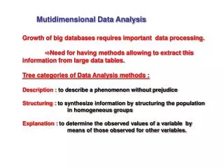
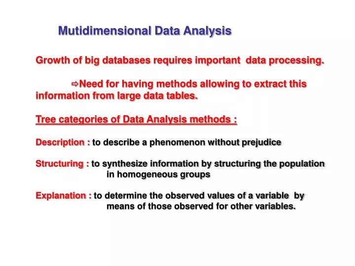
1. Mutidimensional Data Analysis Growth of big databases requires important data processing. Need for having methods allowing to extract this information from large data tables. Tree categories of Data Analysis methods : Description : to describe a phenomenon without prejudice Structuring : to synthesize information by structuring the population in homogeneous groups Explanation : to determine the observed values of a variable by means of those observed for other variables.

2. Mutidimensional Data Analysis one-dimensional descriptive statistics: summarize information for each character. Data Analysis : describe relations between characters and their effects on the structuring of the population. Principal Component Analysis (PCA) Factorial correspondences analysis (FCA)

3. Principal Component Analysis PCA is used when we have a measure data table. Here an example of a measure data file. : Columns : quantitative variables Rows : observations

4. Principal Component Analysis Objectives of the ACP : locate homogeneous groups of observations, across from the set of variables. A large number of variables can be systematically reduced to a smaller, conceptually more coherent set of variables. From the set of the initial statistical variables we can build explicative artificial statistical variables. The principal components are a linear combination of the original variables. Its goal is to reduce the dimensionality of the original data set. A small set of uncorrelated variables is much easier to understand and use in further analyses than a large set of correlated variables.

5. Principal Component Analysis 3 types of PCA General PCA : apply PCA method to the initial Data Table. Centered PCA : apply PCA method to the centered variables. reduced PCA : apply PCA method to the centered and reduced variables

6. Principal Component Analysis - Centered PCA X : statistical variable (Mean of X) (Centered variable)

7. Principal Component Analysis Reduced PCA (Centered and reduced variable)

8. Principal Component Analysis The PCA provides a method of representation of a population in order to Locate homogeneous groups of observations, across from the variables. Reveal differences between observations or groups of observations, across from the set of variables. Highlight observations with the atypical behavior. Reduce the information which allows to describe the position of an observation in the set of the population.

9. Principal Component Analysis Principle The population defined variables on the population. Example:

10. Principal Component Analysis Two types of analysis Analysis of the observations. Analysis of the variables. The reduced analysis:

11. Principal Component Analysis Observations analysis Each observation is represented by a point in a three dimensional space. How to compute a distance between two observations?

12. Principal Component Analysis Observations analysis The 3 axes are defined by variables Y1(.), Y2(.) and Y3(.) calculated from initial variables The distance between two observations i and k is given by : The distance measures the resemblance between these two observations. More the distance is small more the two points are nearby and thus more the two observations resemble each other. Conversely, more the distance is large, more the points are distant and less the observations resemble each other.

13. Principal Component Analysis Observations analysis It is impossible to carry out a representation of the observations in a dimensional space greater than 3. It is thus necessary to find a good representation of the observations group in a space of lower size (2 for example). How to pass from a space of size greater or equal to 3 at a space of more restricted size?  Look for a "good subspace" of representation by using a mathematical operator. Two problems are posed : Give a meaning to the expression "good representation", Characterize the subspace

14. Principal Component Analysis Observations analysis To find under space F such that the distance between points is preserved in the process of projection on this subspace. Thus, the resemblance between observations is preserved in this operation of projection Find a sub-space F such as :

15. Principal Component Analysis Observations analysis Solution : To determine the subspace F, of dimension q, by determining q first eigenvalues and q eigenvectors associated of the matrix Y' Y (Correlation matrix)

16. Principal Component Analysis Observations analysis Z=Y’.Y 1, 2, 3 …. m : Eigenvalues of Z u1, u2, u3 …. um : Eigenvectors of Z Z. u1 : Vector of the n observations coordinates on the first principal axis Z. u2 : Vector of the n observations coordinates on the second principal axis ……….. Z. um : Vector of the n observations coordinates on the mth principal axis

17. Principal Component Analysis Observations analysis It is necessary to build indicators to know quality of the obtained results. These indicators are : an indicator of global quality an indicator of contribution of the observationto total inertia an indicator of contribution of the observationto the inertia explained by the subspace F an indicator of error of perspective.

18. Principal Component Analysis Observations analysis Global quality Eigenvalues of Y'Y : 1 = 0.689 2 = 0.310 3 = 0.00 q : subspace dimension n : number of variables Eigenvalues numbered in the descending order The One dimensional Subspace F : we obtain IQG(F) = 0.6896. The first axis (of the analysis) provide 68.96% of initial information. The subspace generated by the two first axis : IQG(F)=1. (100% of initial info.)

19. Principal Component Analysis Observations analysis Contribution of the observation to total inertia N : number of individuals (observations) in the CPA  CIT(i) = 1. CIT allows to locate easily the observations far distant from center of gravity.

20. Principal Component Analysis Observations analysis contribution of the observation to the inertia explained by the subspace CIE values for nine observations of our example. The CIE determines the observations which contribute more to create a subspace F. In general, this parameter is calculated for all the observations for each axis

21. Principal Component Analysis Observations analysis Error of perspective: The quality of representation of an observation on the subspace COS2(.,.) has the following properties :

22. Principal Component Analysis Variables analysis Objective: to determine synthetic statistical variables which "explain" the initial variables. Problem: to fix the criterion which allows to determine these synthetic variables, then to interpret these variables. In our example, the problem can be posed mathematically as following : Y1(.), Y2(.) and Y3(.) are explained linearly by the synthetic variables Z1(.) and Z2 (.) d1 (.), d2 (.) and d3 (.) are the residual variables, which one want to minimize the variances aij are the solutions of the optimization problem : Min ( V((d1(.))+V(d2(.))+V(d3(.))) V(di(.) : variance of di(.)

23. Principal Component Analysis Variables analysis Solution : calculation of the eigenvectors associated to q greater eigenvalues of matrix YY ' Notice : Matrix YY' has the same no null eigenvalues as the matrix Y' Y. These two eigenvectors define the two sought synthetic variables.

24. Principal Component Analysis Variables analysis The same previous indicators are used in the variables analysis. A significant indicator is IQG(F), the indicator of quality of the subspace F (in which the variables are projected). This indicator allows to calculate the "residual variance” (not taken into account in the representation by the subspace): Residual variance = m.[1 - IQG(F)]

25. Principal Component Analysis Variables analysis it is shown that the coordinate of the projection of a variable on an axis of the subspace is proportional to the linear coefficient of correlation between this variable and the "synthetic" variable corresponding to the axis:¶ Note: Taking into account this proportionality, the program carries out a calculation of reduction which involves that the co-ordinates of projected variables on each axis are directly the linear coefficients of correlation.

26. Principal Component Analysis Variables analysis • For each variable, the coefficient of multiple correlation with the variables corresponding to the axes of a subspace F on which it is projected is proportional to the square of the norm of the projected vector. • A variable will be explained better by the axis of a subspace when the norm of the projected associated vector is large.

27. Principal Component Analysis Simulated example Number of variables : 8 Number of observation : 300

28. Linear correlation between the variables ¶

29. Variables non correlated with X1

30. Les valeurs propres --- Eigenvalues - Cumulated - Cumulated percentage 1 4.09407 4.09407 0.51176 2 3.90593 8.00000 1.00000 3 0.00000 8.00000 1.00000 4 0.00000 8.00000 1.00000 5 0.00000 8.00000 1.00000 6 0.00000 8.00000 1.00000 7 0.00000 8.00000 1.00000 8 0.00000 8.00000 1.00000 100% of inertia is obtained with the two first axes

31. Variables coordinates #2 1 U1 U2 X1 0.7150.699 X2 0.7150.699 X3 -0.715 -0.699 X4 -0.715 -0.699 X5 -0.715 0.699 X6 -0.715 0.699 X7 -0.715 0.699 X8 0.715 -0.699 X5 X6 X1 X2 X7 -1 0 1 #1 X3 U1 : First principal component X4 X8 All the variables are located inside a unit circle (Reduced ACP) -1

32. Variables coordinates #2 1 X5 X6 X1 two dimensions are highlighted X2 X7 -1 0 1 #1 X3 X4 X8 -1

33. observations coordinates

34. Factorial Correspondences Analysis The factorial correspondences analysis is used to extract information starting from the contingency tables. contingency tables (Frequency tables) : crossing of 2 variables X and Y. X : m modalities Y : p modalities Objectives of FCA To build a modalities map of two variables X and Y. To determine if there are correlations between certain modalities of X and some modalities of Y.

35. Factorial Correspondences Analysis Example : 2 variables : ward and expenditure. 5 wards (division in hospital) 5 expenditures (post of expenditure)

36. Factorial correspondences Analysis Analysis of row modalities A row modality is represented by a point of a p dimensions space (27 18 12 19 8) represents second row Row 2 : Point of R5 A rowmodality : 5 points in 5 dimensions space

37. Factorial Correspondences Analysis How to find a subspace of reduced size Q (q=2 for example) to represent these points? The distance between "points represented" (in the subspace) must be the nearest distance between the initial points.  one must define a distance between the points (between modalities). A row modality is represented by a vector Xi whose his coordinates are computed by :

38. Factorial Correspondences Analysis Distance between two modalities is given by : This distance is called Chi-square distance Example : distances between modalities of wards are given in this table :

39. Factorial Correspondences Analysis The problem formulation Find a q-dimensional subspace F, where : is maximized

40. Factorial Correspondences Analysis Center of gravity of xI having a weight fl. Centering operation Each vector zi has p coordinates noted zij. We can define a Matrix Z where the general term is : zij It is shown that the q-dimensional subspace F is generated by the eigenvectors of the matrix Z' Z

41. Factorial Correspondences Analysis Example : Center of gravity Matrix Z Vector xi Vector yi Eigenvalues : 1 = 0.01 2 = 0.00176 3 = 0

42. Factorial Correspondences Analysis Quality of representation indicators Quality of sub-space engendered : q : dimension of sub-space P : number of column modalities

43. Factorial Correspondences Analysis Contribution of a row modality i to making axis k: 0  CIE(i,uk)  1. Example : Contribution of row modalities if CIE is close to 1, the rowmodality has a significant weight in the determination of the subspace F.

44. Factorial Correspondences Analysis Quality of representation (perspective effect) : measure the degree of deformation during projection.

45. Factorial Correspondences Analysis Columns modalities analysis : Columns modalities are analyzed same manner as the rows modalities. Coordinates of xi are such as: The matrices Z' Z and ZZ' have the same ones no null eigenvalues

46. Factorial Correspondences Analysis These indicators have the same definitions, adapted to the columns modalities contributions of columns modalities quality of representation of columns modalities

47. Factorial Correspondences Analysis the simultaneous representation of the rows and the columns projected in the first factorial plane (axes 1 and 2) of our example

48. Illustrations