Download
1 / 64
670 likes | 908 Views
Quantum Control Synthesizing Robust Gates. T. S. Mahesh Indian Institute of Science Education and Research, Pune. Contents. DiVincenzo Criteria Quantum Control Single and Two- qubit control Control via Time-dependent Hamiltonians Progressive Optimization Gradient Ascent

E N D
Quantum Control Synthesizing Robust Gates T. S. Mahesh Indian Institute of Science Education and Research, Pune
Contents • DiVincenzo Criteria • Quantum Control • Single and Two-qubit control • Control via Time-dependent Hamiltonians • Progressive Optimization • Gradient Ascent • Practical Aspects • Bounding within hardware limits • Robustness • Nonlinearity • Summary
Criteria for Physical Realization of QIP • Scalable physical system with mapping of qubits • A method to initialize the system • Big decoherence time to gate time • Sufficient control of the system via time-dependent Hamiltonians • (availability of a universal set of gates). • 5. Efficient measurement of qubits DiVincenzo, Phys. Rev. A 1998
Quantum Control Given a quantum system, how best can we control its dynamics? • Control can be a general unitary or a state to state transfer • (can also involve non-unitary processes: eg. changing purity) • Control parameters must be within the hardware limits • Control must be robust against the hardware errors • Fast enough to minimize decoherence effects • or combined with dynamical decoupling to suppress decoherence
General Unitary General unitary is state independent: Example: NOT, CNOT, Hadamard, etc. Hilbert Space 1 UTG UEXP obtained by simulation or process tomography 0 Fidelity = Tr{UEXP·UTG} / N 2
State to State Transfer A particular input state is transferred to a particular output state Eg. 000 ( 000 + 111 ) /2 Hilbert Space Target Final obtained by tomography Initial Fidelity = FinalTarget 2
Universal Gates • Local gates (eg. Ry(), Rz()) and CNOT gates together form a universal set • Example: Error Correction Circuit • Chiaverini et al, Nature 2004
Degree of control Fault-tolerant computation - E. Knill et al, Science 1998. Quantum gates need not be perfect Error correction can take care of imperfections For fault tolerant computation: Fidelity ~ 0.999
Single Qubit (spin-1/2) Control (up to a global phase) Bloch sphere
~ NMR spectrometer RF coil Pulse/Detect Sample resonance at 0 =B0 B0 Superconducting coil B1cos(wrft)
~ Control Parameters Chemical Shift 01 = 0 - ref All frequencies aremeasured w.r.t. ref RF offset = = rf- ref 1 = B1 rf (kHz rad) B0 RF duration 1 RF amplitude RF phase RF offset B1cos(wrft) time
Single Qubit (spin-1/2) Control (in RF frame) (in REF frame) 90x y x y 90-x A general state: Bloch sphere (up to a global phase)
Single Qubit (spin-1/2) Control (in RF frame) (in REF frame)
Single Qubit (spin-1/2) Control (in RF frame) (in REF frame) Turning OFF 0 : Refocusing Refocus Chemical Shift y X x time w01
Two Qubit Control Local Gates
Qubit Selective Rotations - Homonuclear Band-width 1/ = 1 non-selective 1 2 1 2 = 1 selective dibromothiophene Not a good method: ignores the time evolution
~ ~ Qubit Selective Rotations - Heteronuclear 13CHCl3 1H (500 MHz @ 11T) 13C (125 MHz @ 11T) • Larmor frequencies are separated by MHz • Usually irradiated by different coils in the probe • No overlap in bandwidths at all • Easy to rotate selectively
Two Qubit Control Local Gates CNOT Gate
Two Qubit Control Chemical shift Chemical shift Coupling constant Refocussing: 1 1 Refocus Chemical Shifts Refocus 0 & J-coupling X X 2 2 Rz(90) = 1/(4J) Rz(90) • Rz(0) Z X time time
Two Qubit Control Chemical shift Chemical shift Coupling constant R-z(90) X X H Z H 1/(4J) 1/(4J) time = R-y(90) R-z(90) R-y(90) X =
Control via Time-dependent Hamiltonians H = H (a (t), b (t), g (t) , ) a (t) t NOT EASY !! (exception: periodic dependence)
Control via Piecewise Continuous Hamiltonians a3 a4 a1 a2 b2 b1 b3 b4 g4 g3 g2 g1 Time H 2 H 3 H 4 H 1
Numerical Approaches for Control Progressive Optimization Gradient Ascent NavinKhanejaet al, JMR 2005 D. G. Cory & co-workers, JCP 2002 Mahesh & Suter, PRA 2006 Common features Generate piecewise continuous Hamiltonians Start from a random guess, iteratively proceed Good solution not guaranteed Multiple solutions may exist No global optimization
Piecewise Continuous Control D. G. Cory, JCP 2002 Strongly Modulated Pulse (SMP) (t3,w13,f3,w3) … (t1,w11,f1,w1) (t2,w12,f2,w2)
Progressive Optimization D. G. Cory, JCP 2002 Random Guess Maximize Fidelity simplex Split Maximize Fidelity simplex Split Maximize Fidelity simplex
Example Shifts: 500 Hz, - 500 Hz Coupling: 20 Hz Target Operator : (/2)y1 Fidelity : 0.99
Shifts: 500 Hz, - 500 Hz Coupling: 20 Hz Target Operator : (/2)y1
Shifts: 500 Hz, - 500 Hz Coupling: 20 Hz Target Operator : (/2)y1 Initial state Iz1+Iz2 SMPs are not limited by bandwidth
Shifts: 500 Hz, - 500 Hz Coupling: 20 Hz Target Operator : (/2)y1 Initial state Iz1+Iz2 SMPs are not limited by bandwidth
O CH3 C 2 3 1 C -O H NH3+ 1 2 3 0.99 Pha (deg) Amp (kHz) 0.99 Pha (deg) Amp (kHz) 0.99 Pha (deg) Amp (kHz) Time (ms) 13C Alanine
Benchmarking 12-qubits • Benchmarking circuit A 8 A’ AA’ 2 11 1 1 2 3 3 10 5 4 Qubits 4 7 9 5 6 6 7 8 9 10 Time 11 • PRL, 2006 Fidelity: 0.8
Quantum Algorithm for NGE (QNGE) : in liquid crystal PRA, 2006
Quantum Algorithm for NGE (QNGE) : Quantum Algorithm for NGE (QNGE) : Crob: 0.98 PRA, 2006
Progressive Optimization D. G. Cory, JCP 2002 Advantages Works well for small number of qubits ( < 5 ) Can be combined with other optimizations (genetic algorithm etc) Solutions consist of small number of segments – easy to analyze Disadvantage 1. Maximization is usually via Simplex algorithms Takes a long time
SMPs : Calculation Time During SMP calculation: U = exp(-iHeff t) calculated typically over 103 times QubitsCalc. time 1 - 3 minutes 4 - 6 Hours > 7 Days (estimation) Single ½ : Heff = 2 x 2 Two spins : Heff = 4 x 4 . . . Matrix Exponentiation is a difficult job - Several dubious ways !! 210 x 210 ~ Million 10 spins : Heff =
Gradient Ascent NavinKhanejaet al, JMR 2005 Liouville von-Neumaneqn Control parameters Final density matrix:
Gradient Ascent NavinKhanejaet al, JMR 2005 Correlation: Backward propagated opeartor at t = jt Forward propagated opeartor at t = jt
Gradient Ascent NavinKhanejaet al, JMR 2005 ? = ’ t (up to 1st order in t) ’ ’ ’
Gradient Ascent NavinKhanejaet al, JMR 2005 Step-size
Gradient Ascent NavinKhanejaet al, JMR 2005 GRAPE Algorithm Guess uk No Correlation > 0.99? Yes Stop
Practical Aspects Bounding within hardware limits Robustness Nonlinearity
Bounding the control parameters Quality factor = Fidelity + Penalty function Shoots-up if any control parameter exceeds the limit To be maximized
Practical Aspects Bounding within hardware limits Robustness Nonlinearity
Incoherent Processes Spatial inhomogeneities in RF / Static field Hilbert Space Final Final Final Initial UEXPk(t)
Robust Control Coherent control in the presence of incoherence: Hilbert Space Target Initial UEXPk(t)
Inhomogeneities SFI Analysis of spectral line shapes RFI Analysis of nutation decay SFI Ideal f f z z RFI Ideal y y x x
RF inhomogeneity 1 Ideal Probability of distribution In practice RFI: Spatial nonuniformity in RF power 0 RF Power Desired RF Power
RF inhomogeneity Bruker PAQXI probe (500 MHz)
Example Shifts: 500 Hz, - 500 Hz Coupling: 20 Hz Target Operator : (/2)y1