Download
1 / 37
540 likes | 1.16k Views
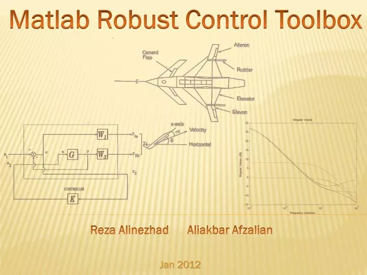
Matlab Robust Control Toolbox. Reza Alinezhad Aliakbar Afzalian. Jan 2012. Outline. Modeling uncertainty Uncertain Elements Uncertain Matricies and Systems Manipulation of Uncertain Models Generalized Robustness Robustness Analysis Performance Analysis

E N D
Matlab Robust Control Toolbox Reza AlinezhadAliakbarAfzalian Jan 2012
Outline • Modeling uncertainty • Uncertain Elements • Uncertain Matricies and Systems • Manipulation of Uncertain Models • Generalized Robustness • Robustness Analysis • Performance Analysis • General control configuration with uncertainty • Interconnection in classic configuration • P-K configuration • N configuration • M-Delta configuration • Robust controller design • Loop shaping • Advance loop shaping • Mu-synthesis with D-K iteration method Reza Alinezhad Aliakbar Afzalian
Modeling Uncertainty Arises when system gains or other parameters are not precisely known, or can vary over a given range Uncertain Elements • UComplex() is a function to define complex uncertain parameters • Ureal() is a function to define real uncertain parameters used in various analysis and design functions in the robust control toolbox. • Ultidyn() is a function to create an uncertain linear time inveriant object where only bounds on the frequency response are known. • Uss() creates uncertain state space objects given the uncertain state space system matriciesa,b,c,d. Reza AlinezhadAliakbarAfzalian
Ureal(‘Name’,Nominal Value) Ureal() is a function to define real uncertain parameters used in various analysis and design functions in the robust control toolbox. Reza Alinezhad Aliakbar Afzalian
Example a = ureal('a',3) Uncertain Real Parameter: Name a, NominalValue 3, variability = [-1 1] get(a) Name: 'a' NominalValue: 3 Mode: 'PlusMinus' Range: [2 4] PlusMinus: [-1 1] Percentage: [-33.3333 33.3333] AutoSimplify: 'basic' Reza Alinezhad Aliakbar Afzalian
UComplex(‘Name’,nominal value) UComplex() is a function to define complex uncertain parameters >> a = ucomplex('a',2-j) Uncertain Complex Parameter: Name a, NominalValue 2-1i, Radius 1 >> get(a) Name: 'a' NominalValue: 2.0000- 1.0000i Mode: 'Radius' Radius: 1 Percentage: 44.7214 AutoSimplify: 'basic Reza Alinezhad Aliakbar Afzalian
Usample(‘Name’,Quantity) USAMPLE Generates random samples of uncertain matrix or... . EX: >> A = ucomplex('A',4+3*j,’Raduse’,1) >> b=usample(A,400); >> plot(b(:),'o'); xlim([0 6]); ylim([1.5 4.5]); EX: >> c = ureal('c',4,'Mode','Range','Percentage',25); >> b=usample(c,400); >> plot(b(:),'o'); xlim([0 500]); ylim([-3 6]); Reza Alinezhad Aliakbar Afzalian
uss(a,b,c,d) Uss() creates uncertain state space objects given the uncertain state space system matriciesa,b,c,d. EX: p1 = ureal('p1',5,'Range',[2 6]); p2 = ureal('p2',3,'Plusminus',0.4); A = [-p1 0;p2 -p1]; B = [0;p2]; C = [1 1]; usys= uss(A,B,C,0) USS: 2 States, 1 Output, 1 Input, Continuous System p1: real, nominal = 5, range = [2 6], 2 occurrences p2: real, nominal = 3, variability = [-0.4 0.4], 1 occurrence Reza Alinezhad Aliakbar Afzalian
Structured uncertainty Uncertainty in an system can occur in various forms and from various sources. Additive Uncertainty Multiplicative Uncertainty Feedback Uncertainty Reza Alinezhad Aliakbar Afzalian
ultidyn('Name',iosize) Uncertain linear, time-invariant objects, ultidyn, are used to represent unknown linear, time-invariant dynamic objects, whose only known attributes are bounds on their frequency response EX: f = ultidyn('f',[1 1]); fsample=usample(f,30); bode(fsample) >> fsample=usample(f) a = f_ultidyn1 f_ultidyn1 -0.4573 b = u1 f_ultidyn1 -0.1707 c = f_ultidyn1 y1 -0.008204 d = u1 y1 0.07623 Reza Alinezhad Aliakbar Afzalian
MAKEWEIGHT(DC,CROSSW,HF) MAKEWEIGHT 1st order system with given DC gain, crossover frequency,and high frequency gain. It must be that |DC| < 1 < |HF|, or |HF| < 1 < |DC|. EX: >> Wi=makeweight(0.15,5,2) >> bode(Wi) a = x1 x1 -8.759 b = u1 x1 4 c = x1 y1 -4.051 d = u1 y1 2 Reza Alinezhad Aliakbar Afzalian
Multiplicative Uncertainty Multiplicative uncertainty isOn of the structured uncertainty that there is rich theory for analyses systems with this type of uncertainty in robust control field. EX: >> a=[0 1;-2 -5]; >> b=[0 1]; >> c=[2 1]; >> d=0; >> sys=ss(a,b',c,d); >> WI=makeweight(0.2,3,2); >> Delta=ultidyn('Delta',[1 1]); >> usys=sys*(1+WI*Delta) USS: 3 States, 1 Output, 1 Input, Continuous System Delta: 1x1 LTI, max. gain = 1, 1 occurrence Reza Alinezhad Aliakbar Afzalian
ufrd(usys,frequency) Ufrd() is a function to create an uncertain frequency response model which often arises when converting uncertain state space objects to frequency response objects. EX: p1 = ureal('p1',5,'Range',[2 6]); p2 = ureal('p2',3,'Plusminus',0.4); p3 = ultidyn('p3',[1 1]); Wt = makeweight(.15,30,10); A = [-p1 0;p2 -p1]; B = [0;p2]; C = [1 1]; usys = uss(A,B,C,0)*(1+Wt*p3); usysfrd = ufrd(usys,logspace(-2,2,60)); bode(usysfrd,'r',usysfrd.NominalValue,'b+') Reza Alinezhad Aliakbar Afzalian
ltiarray2uss(P,Parray,ord) Ltiarray2uss() calculates an uncertain system usys with nominal value P, and whose range of behavior includes the given array of systems, Parray usys = ltiarray2uss(P,Parray,ord) [usys,wt] = ltiarray2uss(P,Parray,ord) [usys,wt,diffdata] = ltiarray2uss(P,Parray,ord) [usys,wt,diffdata] = ltiarray2uss(P,Parray,ord,'InputMult') [usys,wt,diffdata] = ltiarray2uss(P,Parray,ord,'OutputMult') [usys,wt,diffdata] = ltiarray2uss(P,Parray,ord,'Additive') [usys,wt] = ltiarray2uss(P,Parray,ord) usys is formulated as an input multiplicative uncertainty model, usys = P*(I + wt*ultidyn('IMult',[size(P,2) size(P,2)])) where wt is a stable scalar system, whose magnitude overbounds the relative difference, (P - Parray)/P Reza Alinezhad Aliakbar Afzalian
Example: gain = ureal('gain',10,'Perc',20); tau = ureal('tau',.6,'Range',[.42 .9]); wn = 40; zeta = 0.1; usys = tf(gain,[tau 1])*tf(wn^2,[1 2*zeta*wn wn^2]); sysnom = usys.NominalValue; parray = usample(usys,30); om = logspace(-1,2,80); parrayg = frd(parray,om); bode(parrayg) [umodIn1,wtIn1,diffdataIn] = ltiarray2uss(sysnom,parrayg,1); [umodIn2,wtIn2,diffdataIn] = ltiarray2uss(sysnom,parrayg,2); bodemag(wtIn1,'b-',wtIn2,'g+',diffdataIn,'r.',om) Reza Alinezhad Aliakbar Afzalian
Robustness Analysis Reza Alinezhad Aliakbar Afzalian
[stabmarg,destabunc,Report]=robuststab(sys) Robuststab() is used to determine the robust stability margin for a nominally stable uncertain system up to the closest instability from the stable nominal. • Structure Output Fields: • Stabmarg – robust stability margin:lowerbound,upperbound, destabilizing frequency. • Destabunc – structure ofuncertainvalues closesttothenominal thatcauseinstability. • Report – text description of the stability analysis Reza Alinezhad Aliakbar Afzalian
Example: Construct a feedback loop with a second-order plant and a PID controller with approximate differentiation. The second-order plant has frequency-dependent uncertainty, in the form of additive unmodeled dynamics, introduced with an ultidyn object and a shaping filter P = tf(4,[1 .8 4]); delta = ultidyn('delta',[1 1]); Pu = P + 0.25*tf([1],[.15 1])*delta; C = tf([1 1],[.1 1]) + tf(2,[1 0]); S = feedback(1,Pu*C); [stabmarg,destabunc,report] = robuststab(S) Sbad = usubs(S,destabunc); pole(Sbad) ans = 1.0e+002 * -3.2318 -0.2539 -0.0000 + 0.0913i -0.0000 - 0.0913i -0.0203 + 0.0211i -0.0203 - 0.0211i -0.0106 + 0.0116i -0.0106 - 0.0116i stabmarg = UpperBound: 0.8181 LowerBound: 0.8181 DestabilizingFrequency: 9.1321 destabunc = delta: [1x1 ss] Reza Alinezhad Aliakbar Afzalian
[perfmarg,perfmargunc,Report] =robustperf(sys) Robustperf() is a tool to determine the robust performance margin which sets bounds on the robustness of a nominally stable system to given uncertainty. • Structure Output Fields: • Perfmarg – performance margin: lower bound, upper bound, and critical frequency. • Perfmargunc – structure of values of critical uncertain elements of the system. • Report – A text description of the robustness analysis. Reza Alinezhad Aliakbar Afzalian
Example: Create a plant with a nominal model of an integrator, and include additive unmodeled dynamics uncertainty of a level of 0.4. Design a “proportional” controller K that puts the nominal closed-loop bandwidth at 0.8 rad/s. Roll off K at a frequency 25 times the nominal closed-loop bandwidth. Form the closed-loop sensitivity function. P = tf(1,[1 0]) + ultidyn('delta',[1 1],'bound',0.4); BW = 0.8; K = tf(BW,[1/(25*BW) 1]); S = feedback(1,P*K); [perfmargin,punc,report] = robustperf(S) perfmargin = UpperBound: 0.7431 LowerBound: 0.7431 CriticalFrequency: 5.3096 report = Uncertain System achieves a robust performance margin of 0.7431. -- A model uncertainty exists of size 74.3% resulting in a performance margin of 1.35 at 5.31 rad/sec. -- Sensitivity with respect to uncertain element ... 'delta' is 24%. Increasing 'delta' by 25% leads to a 6% decrease in the margin. Reza Alinezhad Aliakbar Afzalian
General Control Configuration With Uncertainty • Iconnect Builds complex interconnections of uncertain matrices and systems. • lft() Generalized feedback interconnection of two LTI models. • lftdata() Decompose uncertain objects into fixed normalized and fixed uncertain parts. • Sysic Builds interconnections of certain and uncertain matrices and systems. Reza Alinezhad Aliakbar Afzalian
P = iconnect • An iconnect object has 3 fields to be set by the user, Input, Output and Equation • Input and Output are icsignal objects, while Equation is a cell-array of equality constraints (using equate) on icsignal objects • the System property is the input/output model, implied by the constraints in Equation relating the variables defined in Input and Output Reza Alinezhad Aliakbar Afzalian
sys = lft(sys1,sys2) sys = lft(sys1,sys2,nu,ny) forms the star product sys of the two LTI models (or LTI arrays) sys1 and sys2.The star product amounts to thefollowing feedback connection for single LTI models (or for each model in an LTI array). • This feedback loop connects the first nu outputs of sys2 to the last nu inputs of sys1 (signals u ), and the last ny outputs of sys1 to the first ny inputs of sys2 (signals y ). The resulting system sys maps the input vector [w1 ; w2] to the output vector [Z1 ;Z2] . Reza Alinezhad Aliakbar Afzalian
Example: Convert classic configuration (fig a) of control problem to general configuration of control problem (fig c). >> D = icsignal(1); >> R = icsignal(1); >> N = icsignal(1); >> U = icsignal(1); >> Z = icsignal(1); >> V = icsignal(1); >> P=iconnect; >> P.input=[D;R;N;U]; >> P.output=[Z;V]; >> P.equation{1}=equate(Z,(rss(3,1,1)*U+rss(2,1,1)*D)-R); >> P.equation{2}=equate(V,(rss(3,1,1)*U+rss(2,1,1)*D)+N); >> Tf(P.System) Reza Alinezhad Aliakbar Afzalian
Example: Transfer function from input 1 to output... 0.08052 s + 0.03601 #1: ----------------------- s^2 + 0.9228 s + 0.1744 -0.2846 s^2 - 0.9822 s - 0.001391 #2: --------------------------------- s^2 + 10.23 s + 27.45 Transfer function from input 4 to output... -0.7805 s^2 - 1.052 s - 0.2911 #1: ------------------------------------- s^3 + 2.156 s^2 + 1.144 s + 2.54e-016 0.3515 s^2 + 0.67 s + 0.2183 #2: ----------------------------------- s^3 + 1.903 s^2 + 0.9427 s + 0.1079 Transfer function from input 2 to output... #1: -1 #2: 0 Transfer function from input 3 to output... #1: 0 #2: 1 Reza Alinezhad Aliakbar Afzalian
Example: >> v=icsignal(1); >> u=icsignal(1); >> K=iconnect; >> K.input=v; >> K.output=u; >> K.equation{1}=equate(u,rss(2,1,1)*v); >> tf(K.System) Transfer function: -0.425 s^2 - 0.7088 s - 0.09289 ------------------------------- s^2 + 1.719 s + 0.2677 >> N=lft(P,K) Transfer function from input 1 to output: -0.01389 s^11 + 0.4599 s^10 + 5.579 s^9 + 23.58 s^8 + 51.58 s^7 + 65.99 s^6 + 51.51 s^5 + 24.47 s^4 + 6.77 s^3 + 0.9771 s^2 + 0.05506 s - 7.075e-007 ------------------------------------------------------------------------------------------------------------------------ s^12 + 17.08 s^11 + 117.5 s^10 + 424.2 s^9 + 908.2 s^8 + 1226 s^7+ 1073 s^6 + 609.4 s^5 + 219.9 s^4 + 47.8 s^3 + 5.618 s^2 + 0.2692 s Reza Alinezhad Aliakbar Afzalian
[M,Delta] = lftdata(A) • Decompose uncertain objects into fixed normalized and fixed uncertain parts • Uncertain objects (umat, ufrd, uss) are represented as certain objects in feedback with block-diagonal concatenations of uncertain elements • separates the uncertain object A into a certain object M and a normalized uncertain matrix Delta such that A is equal to lft(Delta,M), as shown below Ex: >> p1 = ureal('p1',-3,'perc',40); >>p2 = ucomplex('p2',2); >>A = [p1 p1+p2;1 p2]; >>[M,Delta] = lftdata(A) M = 0 0 1.0954 1.0954 0 0 0 1.0000 1.0954 1.0000 -3.0000 -1.0000 0 1.0000 1.0000 2.0000 UMAT: 2 Rows, 2 Columns p1: real, nominal = -3, variability = [-40 40]%, 1 occurrence p2: complex, nominal = 2, radius = 1, 1 occurrence Reza Alinezhad Aliakbar Afzalian
Example EXAMPLE: Create an uncertain matrix A with 2 uncertain real parameters v1 and v2 and create an uncertain system G using A as the dynamic matrix and simple matrices for the input and output A = [ureal('p1',-3,'perc',40) 1;1 ureal('p2',-2)]; sys = ss(A,[1;0],[0 1],0); You can decompose G into a certain system, Msys, and a normalized uncertain matrix, Delta c = x1 x2 y1 1.095 0 y2 0 1 y3 0 1 d = u1 u2 u3 y1 0 0 0 y2 0 0 0 y3 0 0 0 [Msys,Delta] = lftdata(sys) Msys Input groups: Name Channels p1_NC 1 p2_NC 2 Output groups: Name Channels p1_NC 1 p2_NC 2 Delta UMAT: 2 Rows, 2 Columns p1: real, nominal = -3, variability = [-40 40]%, 1 occurrence p2: real, nominal = -2, variability = [-1 1], 1 occurrence a = x1 x2 x1 -3 1 x2 1 -2 b = u1 u2 u3 x1 1.095 0 1 x2 0 1 0 Reza Alinezhad Aliakbar Afzalian
Robust controller design • Loopsyn() is an H – infinity optimal way for loopshaping controller synthisis. • Mixsyn() is H-infinity mixed-sensitivity synthesis method for robust control loopshaping design. • Dksyn() synthesizes a robust controller via D-K iteration which is anapproximationto µ-synthesis control design. Reza Alinezhad Aliakbar Afzalian
[K,CL,GAM,INFO]=loopsyn(G,Gd,RANGE) Loopsyn() is an H – infinity optimal way for loopshaping controller synthisis. • Input Parameters: • G – LTI plant • Gd – desired loop shape • Range – [Wmin,Wmax] desired loop shaping frequency range. (10*Wmin <= Wmax) • Output Parameters: • K – Controller Coefficient vector • CL – Closed Loop System Matrix • Gam – H – infinity norm for the closed loop system • Info – structure containing additional information. EX: s=tf('s'); w0=5; Gd=5/s; G=((s-10)/(s+100))*rss(3,4,5); [K,CL,GAM,INFO]=loopsyn(G,Gd); sigma(G*K,'r',Gd*GAM,'k-.',Gd/GAM,'k-.',{.1,100}) Reza Alinezhad Aliakbar Afzalian
[K,CL,GAM,INFO]=mixsyn(G,W1,W2,W3) Mixsyn() is H-infinity mixed-sensitivity synthesis method for robust control loopshaping design. • Input Parameters: • G – LTI system • W1,W2,W3 – Weighting matricies associated with S(s), R(s) and T(s) • Output Parameters: • K – Controller Coefficient vector • CL – Closed Loop System Matrix • Gam – H – infinity norm for the closed loop system • Info – structure containing additional information. Mixsyn() creates the h-infinity controller based on the sensitivity function S(s) and the complimentatrysensitivitiy T(s) function according to the weighting matricies W1, W2, W3.; Reza Alinezhad Aliakbar Afzalian
K=mixsyn(G,W1,[],W3) With mixsyn controller synthesis, your performance and stability robustness specifications equations are combined into a single infinity norm specification of the form The term is called a mixed-sensitivity cost function because it penalizes both sensitivity S(s) and complementary sensitivity T(s) Loop shaping is achieved when you choose W1 to have the target loop shape for frequencies ω < ωc, and you choose 1/W3 to be the target for ω > ωc. In choosing design specifications W1 and W3 for a mixsyn controller design, you need to ensure that your 0 dB crossover frequency for the Bode plot of W1 is below the 0 dB crossover frequency of 1/W3 Reza Alinezhad Aliakbar Afzalian
Example: NASA HiMAT Design Using MIXSYN >> s=zpk('s'); MS=2;AS=.03;WS=5; W1=(s/MS+WS)/(s+AS*WS); MT=2;AT=.05;WT=20; W3=(s+WT/MT)/(AT*s+WT); [K1,CL1,GAM1]=mixsyn(G,W1,[],W3); L1=G*K1; I=eye(size(L1)); S1=feedback(I,L1); % S=inv(I+L1); T1=I-S1; Figure; sigma(I+L1,'b--',T1,'r:',L1,'r--',W1/GAM1,'y--',GAM1/W3,'k.',{.1,100}) Reza Alinezhad Aliakbar Afzalian
[k,clp,bnd] = dksyn(p,nmeas,ncont) Dksyn() synthesizes a robust controller via D-K iteration which is an approximation to µ-synthesis control design. The objective of μ-synthesis is to minimize the structure singular value μ of the corresponding robust performance problem associated with the uncertain system p The control objective is to synthesize a stabilizing controller k that minimizes the robust performance μ value, which corresponds to bnd. • Input: • P – Partitioned plant matrix • Nmeas – row size of the C2 matrix • Ncon – column size of the B2 matrix • Output: • K – synthesized controller coefficients • Clp – Closed loop system • Bnd – robust performance bounds on the closed loop system Reza Alinezhad Aliakbar Afzalian
Example Let nominal plant model, G, is an unstable first order system G=s/(s-1) >>G = tf(1,[1 -1]); The model itself is uncertain. At low frequency, below 2 rad/s, it can vary up to 25% from its nominal value. Around 2 rad/s the percentage variation starts to increase and reaches 400% at approximately 32 rad/s. >>Wu = 0.25*tf([1/2 1],[1/32 1]); >>InputUnc = ultidyn('InputUnc',[1 1]); The uncertain plant model Gpert represents the model of the physical system to be controlled. >>Gpert = G*(1+InputUnc*Wu); The sensitivity weight Wp has a gain of 100 at low frequency, begins to decrease at 0.006 rad/s, and reaches a minimum of 0.25 after 2.4 rad/s >>Wp = tf([1/4 0.6],[1 0.006]); >> P = [Wp; 1 ]*[1 Gpert]; Reza Alinezhad Aliakbar Afzalian
Example The robustness and performance weights are selected such that if the robust performance structure singular value, bnd, of the closed-loop uncertain system, clp, is less than 1 then the performance objectives have been achieved for all the plant models in the model set. >>[K,clp,bnd] = dksyn(P,1,1); bnd bnd = 0.6860 You can use the robustperf command to analyze the closed-loop robust performance of clp >>[rpnorm,wcf,wcu,report] = robustperf(clp); >>disp(report{1}) Uncertain system, clp, achieves robust performance. The analysis showed clp can tolerate 146% of the model uncertainty and achieve the performance and stability objectives. A model uncertainty exists of size 146% that results in a peak gain performance of 0.686 at 0.569 rad/s Reza Alinezhad Aliakbar Afzalian
References • www.mathworks.com/ • Robust Control Toolbox Tutorial Reza Alinezhad Aliakbar Afzalian